Last updated on：a year ago

Regularization plays an important role in solving the problems of overfitting. I take some notes about it in classes.

Bias/Variance problems

Take mismatched train/test distribution as an example.

Train set error	Dev set error	Remarks
1%	11%	high variance (had too much flexibility to fit)
15%	16%	high bias
15%	30%	high bias + high variance

human 0 %
Optimal/Bayes error: 15%

The basic recipe for ML

High bias (can lead to underfitting), had too much flexibility with high error rate)? (training data performance): Bigger network, training longer, NN architecture search

High variance/overfitting? (dev set performance): more data, regularization, NN architecture search

Bias variance trade-off

Why regularization reduces overfitting

Simplify the neural network, $w^{[l]}$ close to 0

The larger $\lambda$ is, the smaller $w$ is.

$$z^{[l]} = w^{[l]} a^{[l-1]} + b^{[l]}$$

$w^{[l]} \approx 0$, then the last function is becoming a linear function.

Method of regularization

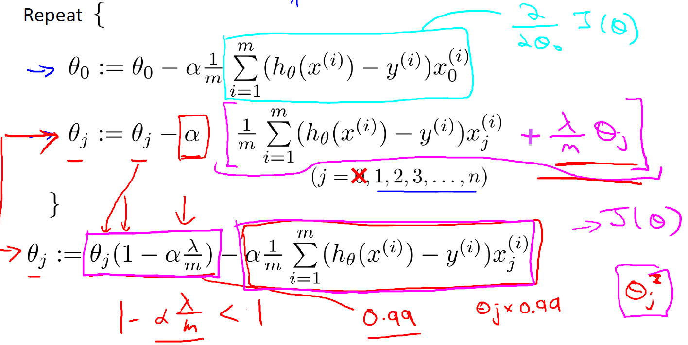
L2 regularization/weight decay

Add the parameters $\theta$/ $w$ into the cost function. $\lambda$ is regularization parameter.

Linear regression

$$J( \theta) = \frac{1}{2m} \left[ \sum_{i=1}^m (h_{\theta} (x^{(i)}) - y^{(i)}) ^2 \right] + \lambda \sum^n_{j=1} \theta_j^2$$

Gradient descent

$\alpha>0, \lambda>0, m>0$

Normal equation

If $\lambda \gt 0$,

$$\theta = \left ( X^T X + \lambda \left [ \begin{matrix}
0 & & & & \\
& 1 & & & \\
& & 1 & & \\ & & & \ddots & \\ & & & & 1 \\
\end{matrix} \right] \right) ^{-1} X^T y$$

Logistic regression

$$J( \theta) = - [\frac{1}{m} \sum_{i=1}^m y^{(i)} \log h_{\theta} (x^{(i)}) + (1- y^{(i)}) \log (1- h_{\theta} (x^{(i)}) )] + \frac{\lambda}{2m} \sum^n_{j=1} \theta_j^2$$

Gradient descent

Repeat:

Compared to linear regression’s, just $$h_\theta (x) = \frac{1}{1 + e^{ - \theta ^T x}}$$

Normal equation: same as linear regression’s

L1 regularization

Compressing the model, $w$ will be sparse

$$\frac{\lambda}{2m} ||w||1= \frac{\lambda}{2m} \sum^{n_x}{i=1} |w|$$

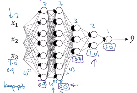
Dropout regularization

Eliminating the nodes of neural network. And it could be different units in the same hidden layer at different times of gradient descent. At the time of test predictions, we usually don’t use dropout.

Intuition: node can’t rely on any single feature, so have to spread out weights.

The size of $w^{[1]}$ should be $7\times 3$.

In general, the number of neurons in the previous layer gives us the number of columns of the weight matrix, and the number of neurons in the current layer gives us the number of rows in the weight matrix.

Data augmentation

It would be redundant sometimes. And the new data is not as good as if you had collected an additional set of brand new independent examples. But you don’t need to pay the expense of going out to take more pictures of cats (an inexpensive way to give you data).

Practical methods: flip horizontally, random crops the image, random distortion, zooming

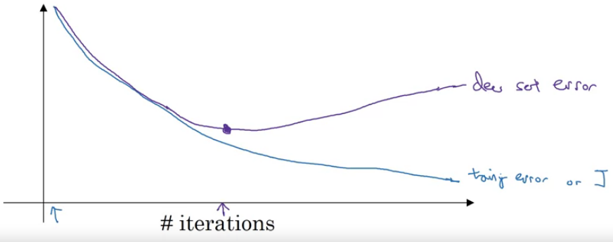
Early stopping

Stop the iterating process in proper time to get a “middle size” $||w||^2_F$. The method is not supposed to be used after fine tuning.

Now, regarding the quantity to monitor: prefer the loss to the accuracy. Why? The loss quantify how certain the model is about a prediction (basically having a value close to 1 in the right class and close to 0 in the other classes). The accuracy merely account for the number of correct predictions. Similarly, any metrics using hard predictions rather than probabilities have the same problem.