Recurrent neural network is widely used in speech recognition, music generation, sentiment classification, DNA sequence analysis, machine translation, video activity recognition, and name entity recognition.

Introduction

Background

Recurrent neural network: Why not a standard networks?

There are problems when handling text:

• Inputs, outputs can be different lengths in different examples

• Doesn’t share features learned across different positions of text

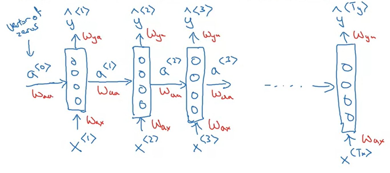
Structure

Input layer: $x^{< t >}$

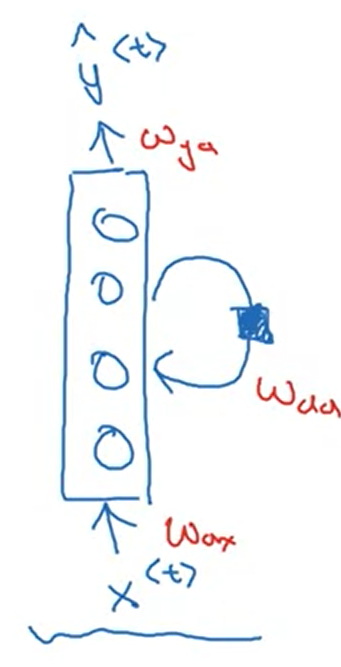
Hidden layer: $a^{< t >}$

Output layer: $\hat{y}^{< t >}$

Shortcomings

It only uses the info that is earlier in the sequence to make a prediction .

Bidirectional RNN (BRNN) can solve the problem.

Notation

$T_x^{(i)}$ length of input sequence

$T_y^{(i)}$ length of output sequence

$x^{(i)< t >}$, the $t$ th sample in the $i$ th input example

$y^{(i)< t >}$, the $t$ th sample in the $i$ th output example

- Superscript $[l]$ denotes an object associated with the $l^{th}$ layer.

- Superscript $(i)$ denotes an object associated with the $i^{th}$ example.

- Superscript $\langle t \rangle$ denotes an object at the $t^{th}$ time step.

- Subscript $i$ denotes the $i^{th}$ entry of a vector.

$a^{(2)[3]<4>}_5$ denotes the activation of the 2nd training example (2), 3rd layer [3], 4th time step <4>, and 5th entry in the vector.

Simplified RNN notation

$$a^{<0>} = 0$$

$a, g(x)$ is tanh/ReLu

$y, g(x)$ is sigmoid

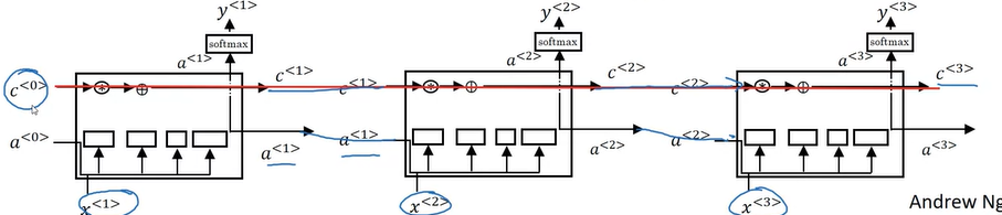
$$a^{< t >} = g(W_{aa} a^{<t - 1>} + W_{ax} x^{< t >} + b_a)$$

$$y^{< t >} = g(W_{ya} a^{< t >} + b_y)$$

Also, $a^{< t >}$ can be represented by:

$$a^{< t >} = g(W_{a} [a^{<t - 1>}, x^{< t >}] + b_a)$$

Here,

$$W_{a} = \left[ W_{aa} W_{ax} \right] $$

Backpropagation through time

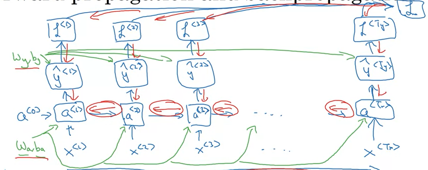
$$\mathcal{L}^{< t >} (\hat{y}^{< t >}, y^{< t >}) = - y^{< t >} \log y^{< t >} - (1 - y^{< t >}) \log (1- y^{< t >})$$

Sum:

$$\mathcal{L} (\hat{y}^{< t >}, y^{< t >}) = \sum_{t=1}^{T_x} \mathcal{L}^{< t >} (\hat{y}^{< t >}, y^{< t >}) $$

Situations when this RNN will perform better

- This will work well enough for some applications, but it suffers from vanishing gradients.

- The RNN works best when each output $\hat{y}^{\langle t \rangle}$ can be estimated using “local” context.

- “Local” context refers to information that is close to the prediction’s time step $t$.

- More formally, local context refers to inputs $x^{\langle t’ \rangle}$ and predictions $\hat{y}^{\langle t \rangle}$ where $t’$ is close to $t$.

What you should remember:

* The recurrent neural network, or RNN, is essentially the repeated use of a single cell.

* A basic RNN reads inputs one at a time, and remembers information through the hidden layer activations (hidden states) that are passed from one time step to the next.

* The time step dimension determines how many times to re-use the RNN cell

* Each cell takes two inputs at each time step:

* The hidden state from the previous cell

* The current time step’s input data

* Each cell has two outputs at each time step:

* A hidden state

* A prediction

Different types

Background

Input and output may have different length, or even types.

Types

One to one: generic neural network

One to many: music generation

Many to one: sentence classification

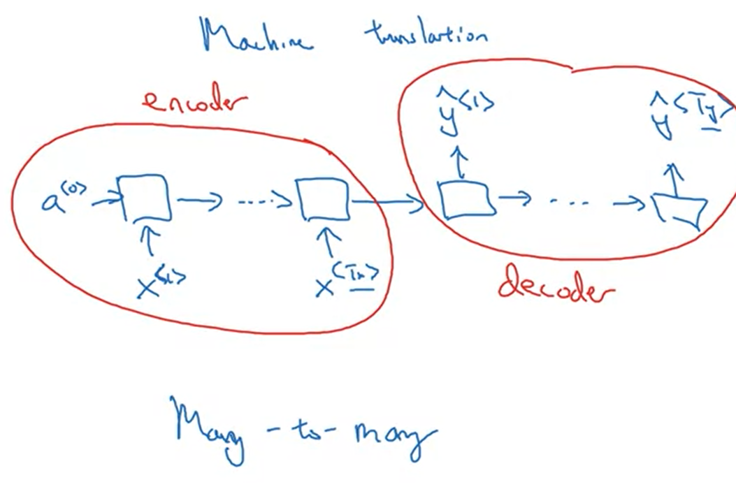
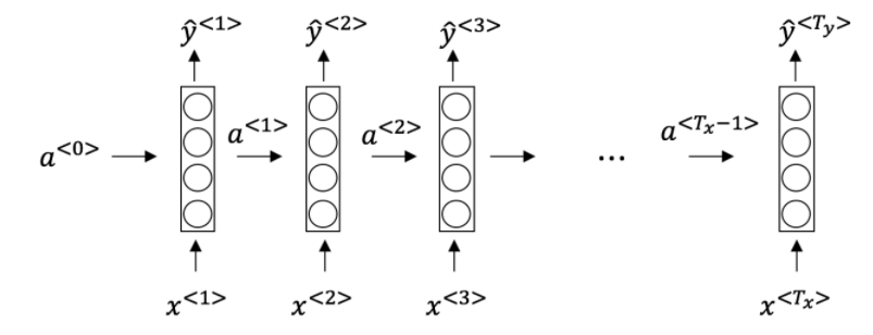
Many to many: $T_x = T_y$

Many to many: $T_x != T_y$

RNN

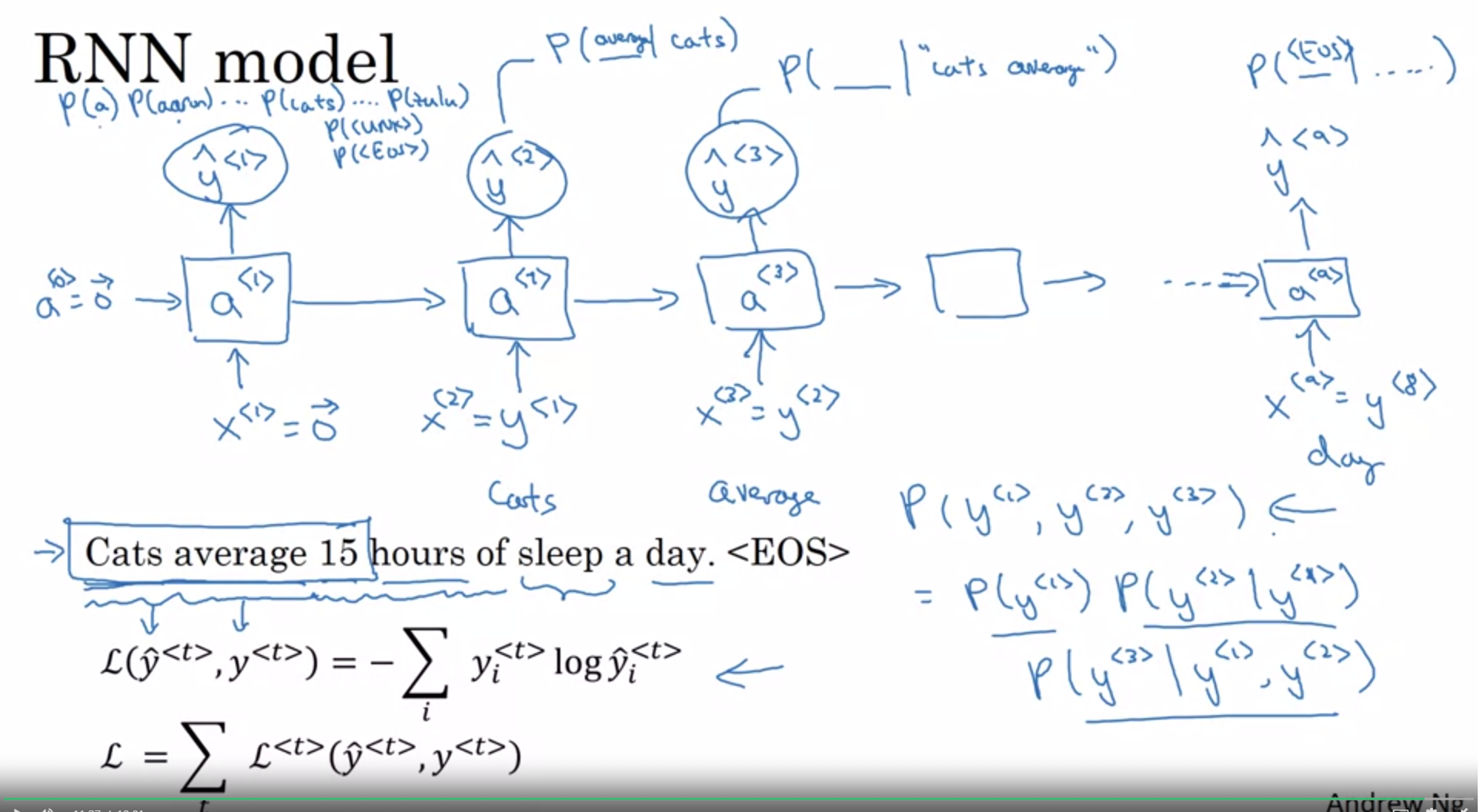
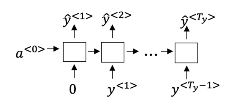
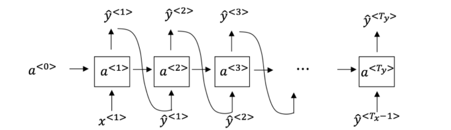
Sample novel sequences

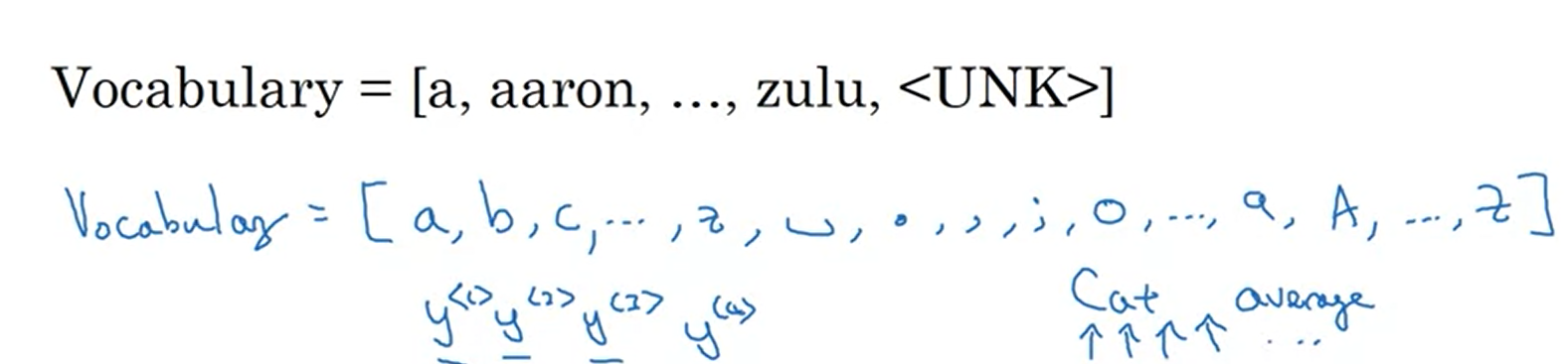
Character-level language model

$y^{< T >}$ will be individual characters

Vocabulary

Don’t ever have to worry about unknown word tokens. It is more computationally expensive

Problems

Vanishing gradient with RNNs: long term dependencies It’s just very difficult for the error to backpropagate all the way to the beginning of the sequence

Exploding gradients, solution: gradient clipping

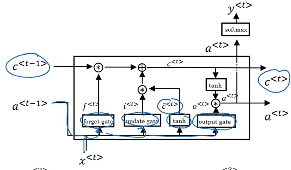
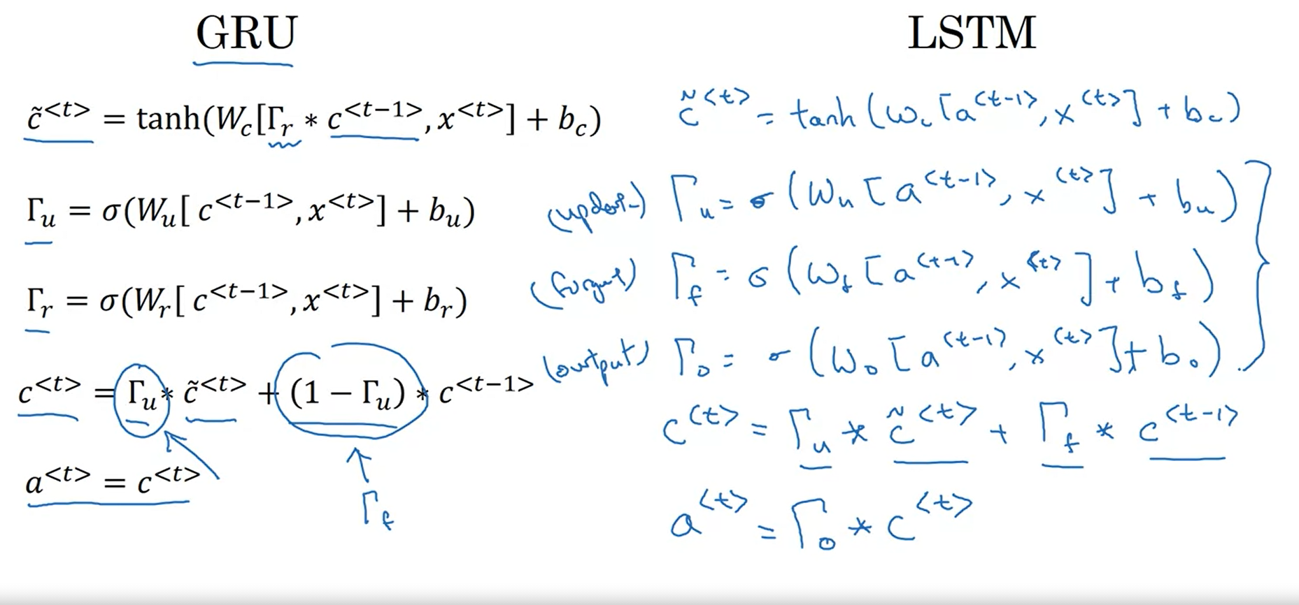
LSTM

LSTM means long short term memory. It is constructed by gate recurrent unit (GRU). LSTM has some value $C_0$ and it passes all the way to the right to have. Maybe $C_3$ equals to $C_0$. That’s why the LSTM as well as the GRU is very good at memorizing certain values. (Peephole connection)

LSTM is more powerful and more flexible since there’s three gates instead of two.

Notation

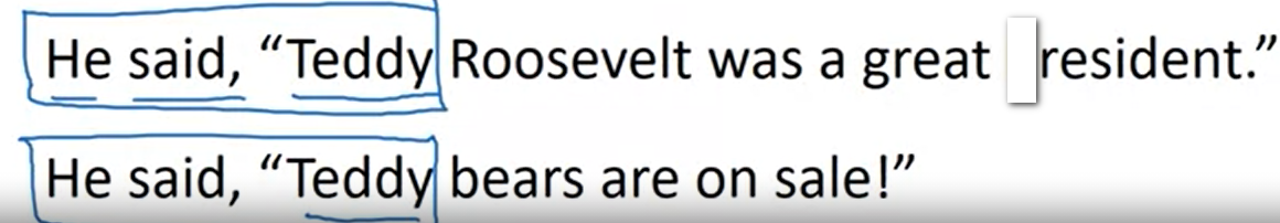
Let’s assume you are reading words in a piece of text, and plan to use an LSTM to keep track of grammatical structures, such as whether the subject is singular (“puppy”) or plural (“puppies”).

If the subject changes its state (from a singular word to a plural word), the memory of the previous state becomes outdated, so you’ll “forget” that outdated state.

• The “forget gate” is a tensor containing values between 0 and 1.

• • If a unit in the forget gate has a value close to 0, the LSTM will “forget” the stored state in the corresponding unit of the previous cell state.
  • If a unit in the forget gate has a value close to 1, the LSTM will mostly remember the corresponding value in the stored state.

BRNN

Bidirectional RNN: use a cyclic graph and take into account the information from the past and from the future.

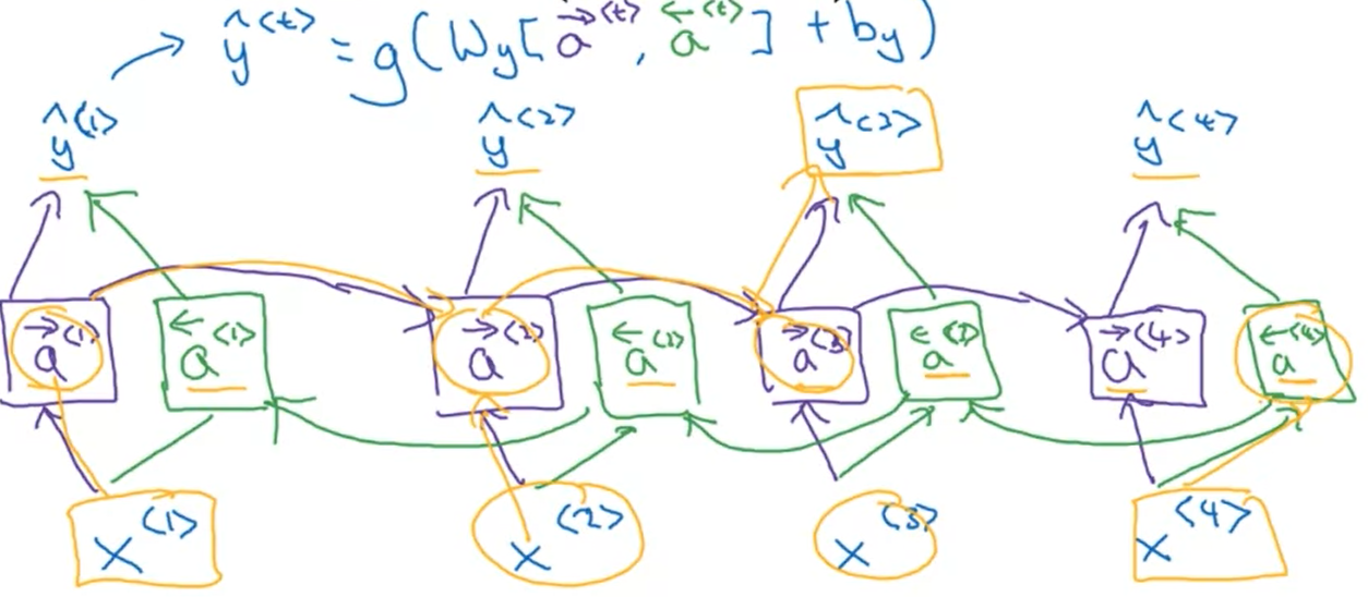
Disadvantage:

Need the entire sequence of data.

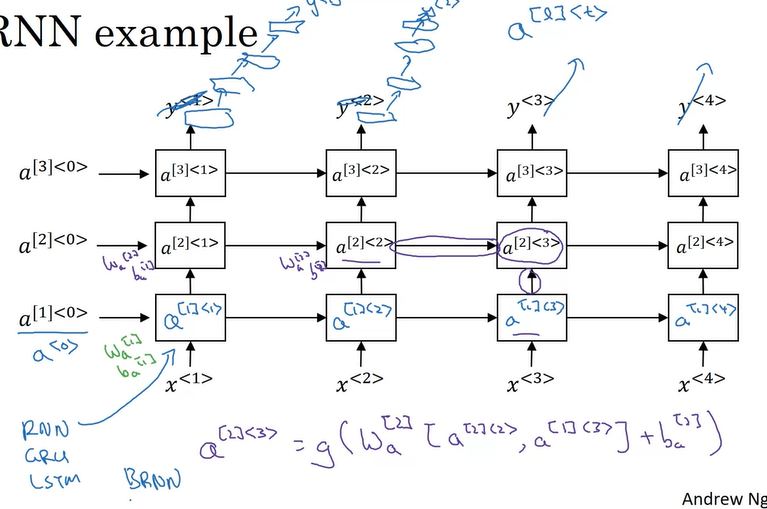
Deep RNNs

$a^{[l]< t >}$

$l$, layer $l$

$t$, time $t$

What you should remember

• Very large, or “exploding” gradients updates can be so large that they “overshoot” the optimal values during back prop – making training difficult

• • Clip gradients before updating the parameters to avoid exploding gradients

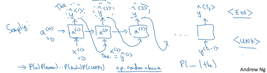
• Sampling is a technique you can use to pick the index of the next character according to a probability distribution.

• • To begin character-level sampling:

  • • Input a “dummy” vector of zeros as a default input
    • Run one step of forward propagation to get $a^{<1>}$ (your first character) and $\hat{y}^{<1>}$ (probability distribution for the following character)
    • When sampling, avoid generating the same result each time given the starting letter (and make your names more interesting!) by using np.random.choice

• A sequence model can be used to generate musical values, which are then post-processed into midi music.

• You can use a fairly similar model for tasks ranging from generating dinosaur names to generating original music, with the only major difference being the input fed to the model.

• In Keras, sequence generation involves defining layers with shared weights, which are then repeated for the different time steps $1,…,T_x$.

• An LSTM is similar to an RNN in that they both use hidden states to pass along information, but an LSTM also uses a cell state, which is like a long-term memory, to help deal with the issue of vanishing gradients

• An LSTM cell consists of a cell state, or long-term memory, a hidden state, or short-term memory, along with 3 gates that constantly update the relevancy of its inputs:

• • A forget gate, which decides which input units should be remembered and passed along. It’s a tensor with values between 0 and 1.

  • • If a unit has a value close to 0, the LSTM will “forget” the stored state in the previous cell state.
    • If it has a value close to 1, the LSTM will mostly remember the corresponding value.

  • An update gate, again a tensor containing values between 0 and 1. It decides on what information to throw away, and what new information to add.

  • • When a unit in the update gate is close to 1, the value of its candidate is passed on to the hidden state.
    • When a unit in the update gate is close to 0, it’s prevented from being passed onto the hidden state.

  • And an output gate, which decides what gets sent as the output of the time step

Q & A

1.Suppose your training examples are sentences (sequences of words). Which of the following refers to the j^{th}jth word in the i^{th}ith training example?

-$[x] x^{(i)< j >}$

$x^{< i >(j)}$

-[ ] $x^{(j)< i >}$

$x^{< j >(i)}$

2.This specific type of architecture is appropriate when:

-[x] $T_x = T_y$

$T_x < T_y$

$T_x > T_y$

$T_x =1$

3.To which of these tasks would you apply a many-to-one RNN architecture? (Check all that apply).

Speech recognition (input an audio clip and output a transcript)

-[x] Sentiment classification (input a piece of text and output a 0/1 to denote positive or negative sentiment)

Image classification (input an image and output a label)

-[x] Gender recognition from speech (input an audio clip and output a label indicating the speaker’s gender)

4.You are training this RNN language model, at the $t$th time step, what is the RNN doing? Choose the best answer.

Estimating $P(y^{<1>}, y^{<2>}, …, y^{< t-1 >})P(y<1>,y<2>,…,y<*t*−1>)$

Estimating $P(y^{< t >})P(y< *t* >)$

-[x] Estimating $P(y^{< t >} \mid y^{<1>}, y^{<2>}, …, y^{< t-1 >})P(y< t* >∣y*<1>,y<2>,…,y<*t*−1>)$

Estimating $P(y^{< t >} \mid y^{<1>}, y^{<2>}, …, y^{< t >})P(y<t*>∣y*<1>,y<2>,…,y<*t*>)$

In a language model we try to predict the next step based on the knowledge of all prior steps.

5.You have finished training a language model RNN and are using it to sample random sentences, as follows:

What are you doing at each time step t?

(i) Use the probabilities output by the RNN to pick the highest probability word for that time-step as $\hat{y}^{< t >}$. (ii) Then pass the ground-truth word from the training set to the next time-step.

-[ ] (i) Use the probabilities output by the RNN to randomly sample a chosen word for that time-step as $\hat{y}^{< t >}$.(ii) Then pass the ground-truth word from the training set to the next time-step.

(i) Use the probabilities output by the RNN to pick the highest probability word for that time-step as $\hat{y}^{< t >}$.(ii) Then pass this selected word to the next time-step.

-[x] (i) Use the probabilities output by the RNN to randomly sample a chosen word for that time-step as $\hat{y}^{< t >}$.(ii) Then pass this selected word to the next time-step.

The ground-truth word from the training set is not the input to the next time-step.

6.Alice proposes to simplify the GRU by always removing the $\Gamma_u$. I.e., setting $\Gamma_u = 1$. Betty proposes to simplify the GRU by removing the $\Gamma_r$. I. e., setting $\Gamma_r = 1$ always. Which of these models is more likely to work without vanishing gradient problems even when trained on very long input sequences?

-[ ] Alice’s model (removing $\Gamma_u$), because if $\Gamma_r \approx 0$ for a timestep, the gradient can propagate back through that timestep without much decay.

-[] Alice’s model (removing $\Gamma_u$), because if $\Gamma_r \approx 1$ for a timestep, the gradient can propagate back through that timestep without much decay.

-[x] Betty’s model (removing $\Gamma_r$), because if $\Gamma_u \approx 0$ for a timestep, the gradient can propagate back through that timestep without much decay.

-[ ] Betty’s model (removing $\Gamma_r$), because if $\Gamma_u \approx 1$ for a timestep, the gradient can propagate back through that timestep without much decay.

For the signal to backpropagate without vanishing, we need $c^{< t >}$ to be highly dependent on $c^{< t-1 >}$.

Reference

[1] Deeplearning.ai, Sequence Models