Metrics used in deep learning
Last updated on:6 months ago
As a researcher in deep learning, we have to make use of metrics to measure our models’ performance. I’ll introduce the most seen metrics in this blog.
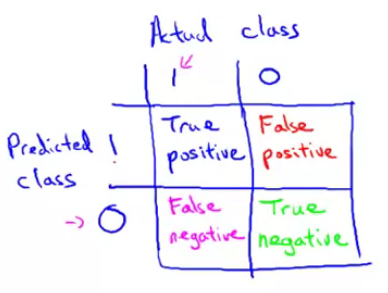
Error matrices
Positive and negative are your judgement result. True or False means your judgement is right or wrong.
Condition positive (P): the number of real positive cases in the data.
Condition negative (N): the number of real negative cases in the data.
True positive (TP): a test result that correctly indicates the presence of a condition or characteristic.
True negative (TN): a test result that correctly indicates the absence of a condition or characteristic.
False positve (FP), type I error: a test result which wrongly indicates that a particular condition or attribute is present.
False negative (FN), type II error: a test result which wrongly indicates that a particular condition or attribute is absent.
Divisor P, N means all positive or negative cases
- Accuracy = (true positives + true negatives) / (total examples)
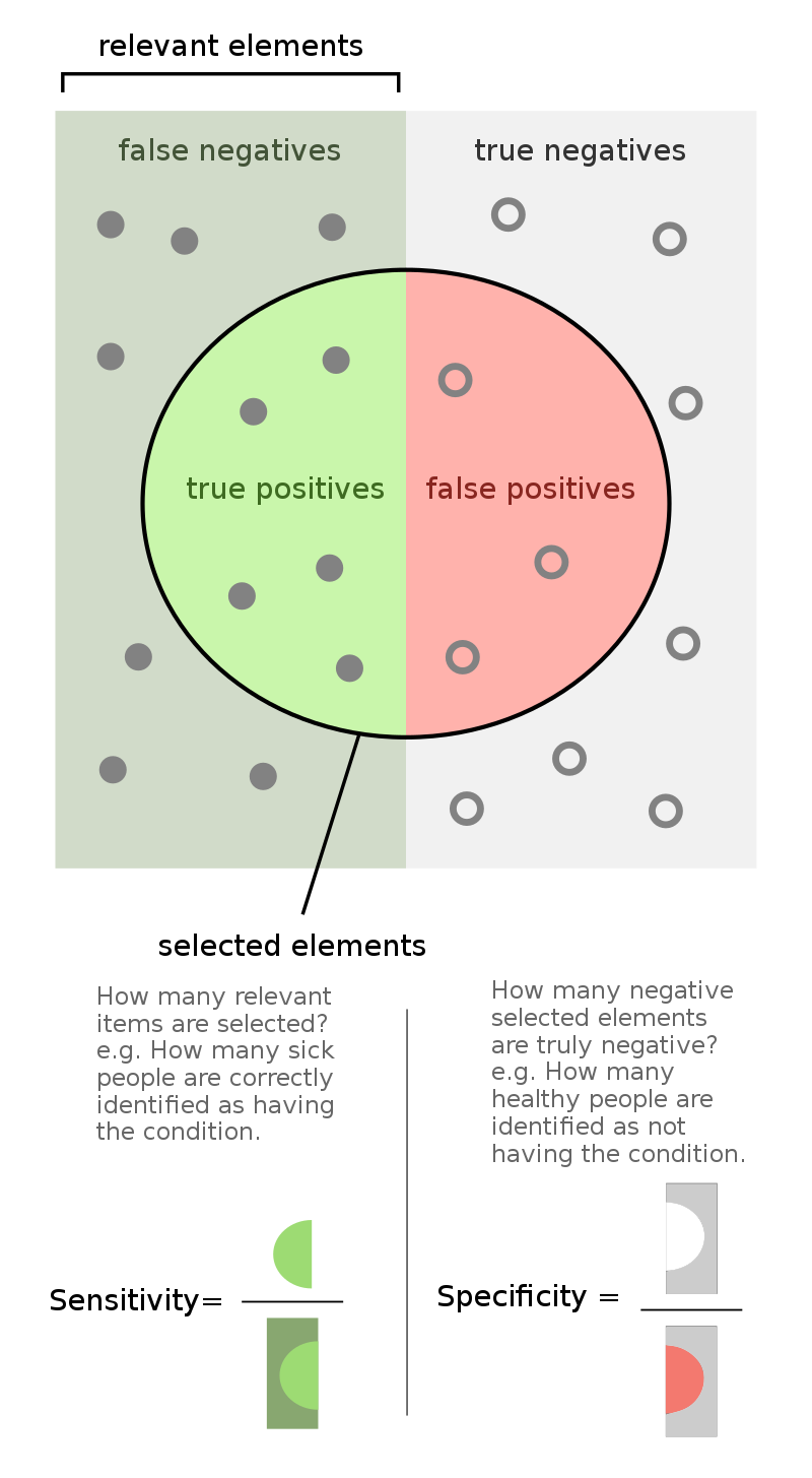
- Precision = (true positives) / (true positives + false positives)
- Recall (or Sensitivity) = (true positives) / (true positives + false negatives)
- F1 score (F score) = $2\frac{PR}{P+R}$ or $\frac{2}{1/P+1/R}$
- Specificity = $\frac{TN}{TN + FP}$
Biomedical meaning
Specificity: Find the healthy guys from all people, not giving miseading message.
Sensitivity: Find the illness guys from all people, giving the timely message.
$F_{\beta }$ score
Emphasize the sensitivity, by giving large $\beta$ value, the impact of precisaion will be smaller.
$${\displaystyle F_{\beta }=(1+\beta ^{2})\cdot {\frac {\mathrm {precision} \cdot \mathrm {recall} }{(\beta ^{2}\cdot \mathrm {precision} )+\mathrm {recall} }}}$$
For instance, if $\beta = 2$, then $F_{2}$ score would be:
$${\displaystyle F_{\beta }=5\cdot {\frac {\mathrm {precision} \cdot \mathrm {recall} }{(4\cdot \mathrm {precision} )+\mathrm {recall} }}}$$
Metrics Rate
Rate means the proportion of an indicator. The fraction of metrics rate is depended on the rate name.
| Rate name | Denominator | Numerator | Formula |
|---|---|---|---|
| True positive rate/TPR | TP + FN | TP | $\frac{TP}{TP + FN}$ |
| False positive rate/FPR | FP + TN | FP | $\frac{FP}{FP + TN}$ |
| True negative rate/TNR | TN + FP | TN | $\frac{TN}{TN + FP}$ |
| False negative rate/FNR | FN + TP | FN | $\frac{FN}{FN + TP}$ |
Denominator is the total of the rate name situation in judgement (positive or negative). For instance, True positive means ground truth and judgement are right. We get all positive judgement item, that is TP $+$ FN. Meanwhile, the numerator is the rate name itself. True positive is TP.
The ground truth and judgement are both different in two rate name means we can sum up them to 1.
$$\text{FPR} + \text{TNR} = 1$$
$$\text{TPR} + \text{FNR} = 1$$
Name
TPR: Sensitivity, Recall
FPR: Fall out
TNR: Specificity, selectivity
FNR: Miss rate
ROC
A receiver operating characteristic curve, or ROC curve, is a graphical plot that illustrates the diagnostic ability of a binary classifier system as its discrimination threshold is varied.
ROC curve is TPR-FPR curve, which means that we need to compute TPR and FPR first.
AUC is area under curve. It can be obtained by calculate the area among ROC curve, $x$ axis, and $y = 1$ axis.
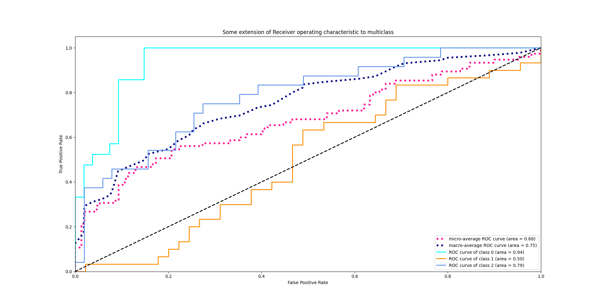
I guess you may have a question about plotting a curve. We get the TPR and FPR result in evaluating process, which can just be plotted in one point. How do we plot this curve? Actually, we need to set a threshold to define how large possibility is taken as a positive judgement.
For multi classes, we plot each class ROC one by one. First binarize the other class and the interested class, then take it as a two class curve plotting problem.
from sklearn.metrics import roc_curve, auc
import matplotlib.pyplot as plt
import numpy as np
from sklearn import metrics
y = np.array([1, 1, 2, 2])
scores = np.array([0.1, 0.4, 0.35, 0.8])
fpr, tpr, thresholds = metrics.roc_curve(y, scores, pos_label=2)
>>> fpr
array([ 0. , 0.5, 0.5, 1. ])
>>> tpr
array([ 0.5, 0.5, 1. , 1. ])
>>> thresholds
array([ 0.8 , 0.4 , 0.35, 0.1 ])
auc = metrics.auc(fpr, tpr)
>>> auc
0.75
plt.figure()
lw = 2
plt.plot(fpr, tpr, color='darkorange',
lw=lw, label='ROC curve (area = %0.2f)' % auc)
plt.plot([0, 1], [0, 1], color='navy', lw=lw, linestyle='--')
plt.xlim([0.0, 1.0])
plt.ylim([0.0, 1.05])
plt.xlabel('False Positive Rate')
plt.ylabel('True Positive Rate')
plt.title('Receiver operating characteristic example')
plt.legend(loc="lower right")
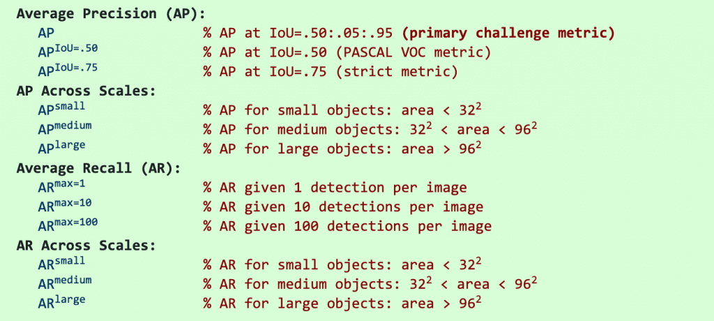
plt.show()Mean average prevision
The general definition for the average precision is the are under the precision-recall curve.
Bugs and problems
It is quite wired that mAP and loss are both smaller during training. I think it is caused by classification loss take place in large part.
Training Loss 和 Validation mAP 剧烈起伏
Not just classification loss dominate localisation loss, but the small anchor is ignored by large min_ratio of length for anchor generator.
MMDetection中,为什么训练到后面几个epoch,mAP减小了?
过拟合了,而且感觉mmdet性能不如原生框架.
https://www.zhihu.com/question/449003051
loss一直降
说明只能说明模型在训练集上性能越来越好 验证集mAP没变可能原因:验证集数据太少 或者 和训练集分布差别太大 或者 模型在训练集上过拟合了。 可以试着在训练集上推理下看下是否过拟合,总之可以通过加大数据集 添加数据增强 调整验证集大小等手段来改善这个现象。
Reference
[1] Receiver operating characteristic
[4] F-score
本博客所有文章除特别声明外,均采用 CC BY-SA 4.0 协议 ,转载请注明出处!