Sometimes, we want our network to be low computational cost at deployment, or useful for mobile and embedded vision applications. In these cases, we can make use of MobileNet to satisfy our expectation.

Depthwise separable convolution

Perform two steps of convolution.

= Depth wise conv + point wise conv

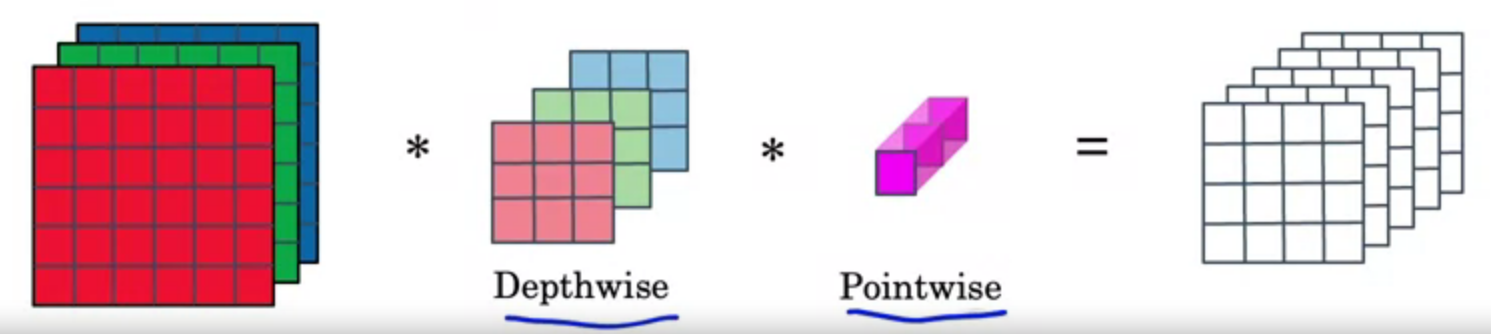
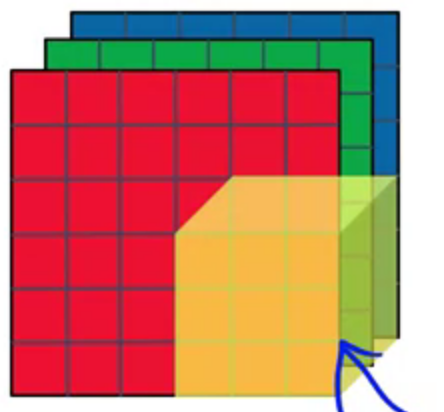
Depth wise

For the “Depthwise” computations each filter convolves with only one corresponding colour channel of the input image.

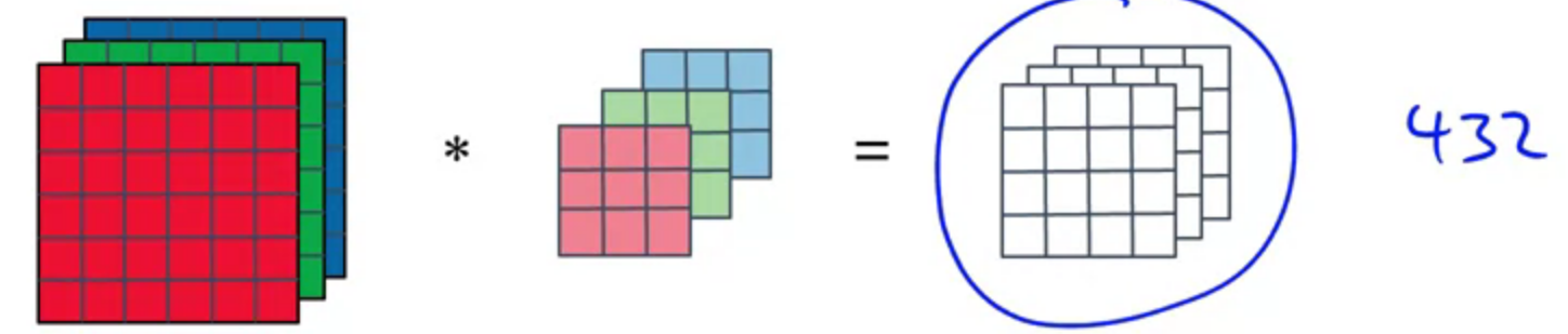
$$n \times n \times n_c * f \times f = n_{out} \times n_{out} \times n_c$$

You convolve the input image with $n_c$ number of $$n_f \times n_f$$ filters $n_c$ is the number of colour channels of the input image].

Point wise

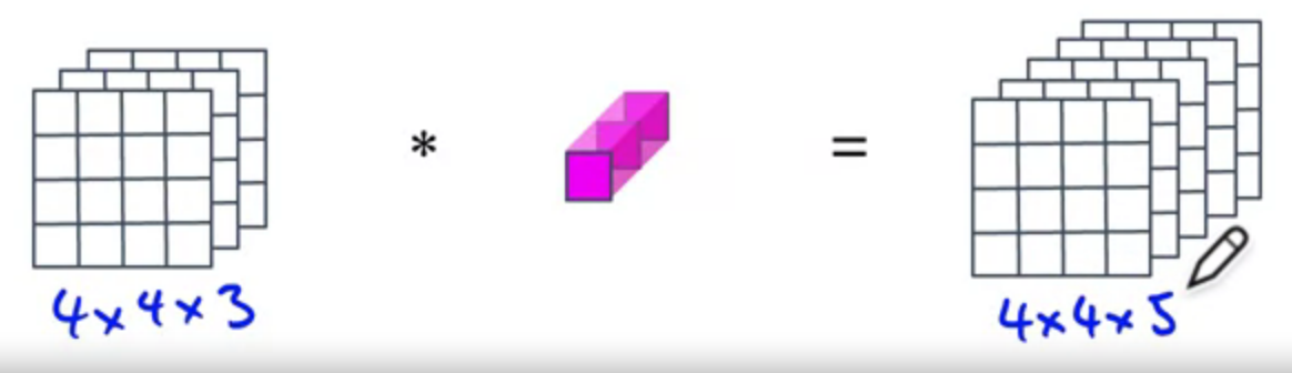
$$n_{out} \times n_{out} \times n_c * 1 \times 1 \times n_c = n_{out} \times n_{out} \times n_c^{‘}$$

The final output is of the dimension $$n_{out} \times n_{out} \times n_c^{‘}$$ (where $n_c^{‘}$ is the number of filters used ln the previous convolution step).

Computational cost

For plain convolution:

Computational cost = $$\text{No. filter params} \times \text{No. filter params} \times \text{No. of filters}$$
Computational cost = $$f \times f \times n_c \times n_{out} \times n_{out} \times n_c^{‘}$$

For depthwise separable convolution:

Computational cost =

$$f \times f \times n_{out} \times n_{out} \times n_c^{‘} + $$

$$n_c \times n_{out} \times n_{out} \times n_c^{‘}$$

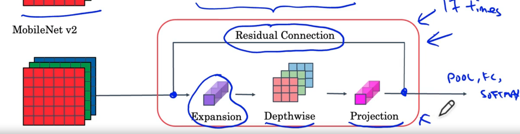
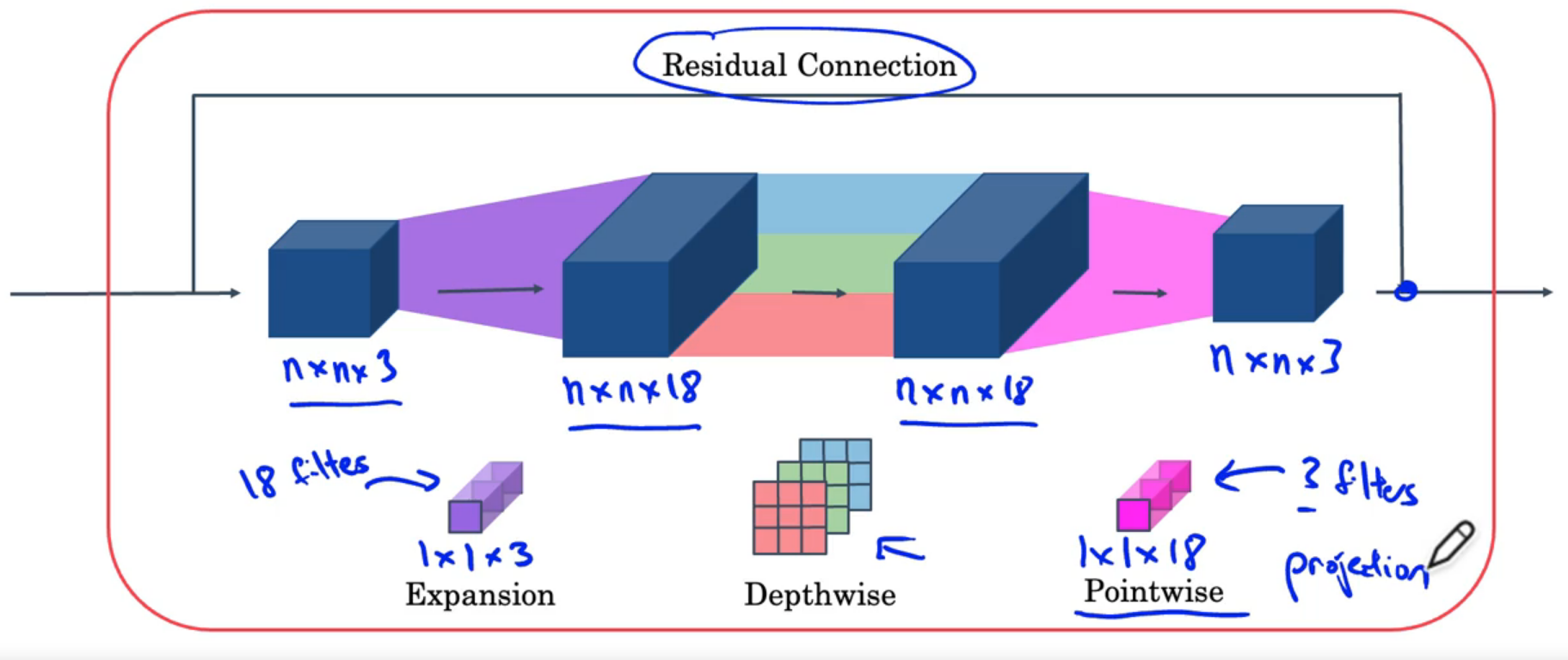
MobileNets

v1

Residual connection, expansion depthwise projection.

Squeeze and excitation

通過全局pooling然後壓縮通道再復原，實現提取global info，利用了attention的原理，然後再用scale方法回乘。

torch.Size([3, 16, 56, 56])
torch.Size([3, 16, 1, 1])
torch.Size([3, 8, 1, 1])
torch.Size([3, 8, 1, 1])
torch.Size([3, 16, 1, 1])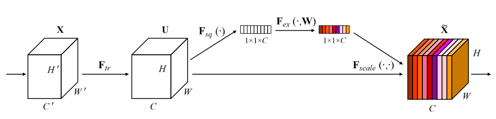

Codes:

class SqueezeExcitation(nn.Module):
    # Implemented as described at Figure 4 of the MobileNetV3 paper
    def __init__(self, input_channels: int, squeeze_factor: int = 4):
        super().__init__()
        squeeze_channels = _make_divisible(input_channels // squeeze_factor, 8)
        self.fc1 = nn.Conv2d(input_channels, squeeze_channels, 1)
        self.relu = nn.ReLU(inplace=True)
        self.fc2 = nn.Conv2d(squeeze_channels, input_channels, 1)
    def _scale(self, input: Tensor, inplace: bool) -> Tensor:
        scale = F.adaptive_avg_pool2d(input, 1)
        scale = self.fc1(scale)
        scale = self.relu(scale)
        scale = self.fc2(scale)
        return F.hardsigmoid(scale, inplace=inplace)
    def forward(self, input: Tensor) -> Tensor:
        scale = self._scale(input, True)
        return scale * input # attention mechanisms, use global info

v2 Bottleneck

Enable the richer computation, keep the amount of memory relatively small

Use open source code

• Use architectures of networks published in the literature
• Use open source implementations if possible
• Use pretrained models and fine-tune on your dataset

Q&A 8

Which of the following are common reasons for using open-source implementations of ConvNets (both the model and/or weights)? Check all that apply.

-[x] It is a convenient way to get working with an implementation of a complex ConvNet architecture.

-[] The same techniques for winning computer vision competitions, such as using multiple crops at test time, are widely used in practical deployments (or production system deployments) of ConvNets.

-[x] Parameters trained for one computer vision task are often useful as pretraining for other computer vision tasks.

-[] A model trained for one computer vision task can usually be used to perform data augmentation

Transfer learning

You could try fine-tuning the model by re-running the optimizer in the last layers to improve accuracy. When you use a smaller learning rate, you take smaller steps to adapt it a little more closely to the new data. In transfer learning, the way you achieve this is by unfreezing the layers at the end of the network, and then re-training your model on the final layers with a very low learning rate. Adapting your learning rate to go over these layers in smaller steps can yield more fine details and higher accuracy.

More complex, high-level features like wispy hair or pointy ears begin to emerge. For transfer learning, the low-level features can be kept the same, as they have common features for most images. When you add new data, you generally want the high-level features to adapt to it, which is rather like letting the network learn to detect features more related to your data, such as soft fur or big teeth.

To achieve this, just unfreeze the final layers and re-run the optimizer with a smaller learning rate, while keeping all the other layers frozen.

What you should remember:

• To adapt the classifier to new data: Delete the top layer, add a new classification layer, and train only on that layer
• When freezing layers, avoid keeping track of statistics (like in the batch normalization layer)
• Fine-tune the final layers of your model to capture high-level details near the end of the network and potentially improve accuracy

Reference

[1] Howard, A.G., Zhu, M., Chen, B., Kalenichenko, D., Wang, W., Weyand, T., Andreetto, M. and Adam, H., 2017. Mobilenets: Efficient convolutional neural networks for mobile vision applications. arXiv preprint arXiv:1704.04861.

[2] Deeplearning.ai, Convolutional Neural Networks