Self-supervised learning learns representations from the physical nature
Last updated on:7 months ago
Self-supervised visual representation learning is a method that learns the physical essence of nature objectives. It is a promising subclass of unsupervised learning. Compared to vanilla unsupervised learning, it uses pre-setting information as the problem of the pretext task.
Introduction
Representation learning is a field to gain insight into the intrinsic nature of object physics. An unsupervised signal is created automatically to learn useful representations for solving real-world downstream tasks.
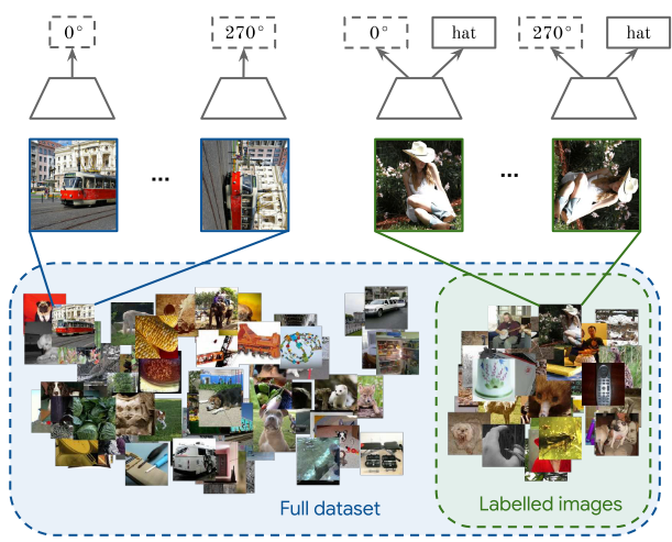
The self-supervised learning framework requires only unlabelled data to formulate a pretext learning task such as predicting context or image rotation. A target objective can be computed without supervision. These pretext tasks must be designed so that high-level image understanding is helpful in solving them.
Architecture choices which negligibly affect performance in the fully labelled setting may significantly affect performance in the self-supervised setting. Skip connections do not degrade towards the end of the model. VGG19-BN deteriorates towards the end of the network. This happens because the models specialise in the pretext task in the later layers and, discard more general semantic features in the middle layers.
But this is not the case for models with skip-connections: representation quality in ResNet consistently increases up to the final pre-logits layer. Skip connections make ResNet invertible under some conditions, as reported by Alexander et al. Invertible units preserve all information learned in intermediate layers and, thus, prevent deterioration of representation quality.
Motivation
Building large labelled datasets for all these scenarios is not practically feasible.
After seeing only a few (labelled) examples, humans can understand new concepts quickly.
Aims
Successfully learn to recognise new concepts by leveraging only a small amount of labelled examples.
The representation from the (frozen) network at the pre-logits level (backbone), but investigate other possibilities (downstream tasks). Alexander et al. use an MLP for solving the evaluation task (classifier).
Downstream tasks: Multiclass image classification tasks requiring high-level scene understanding.
Evaluation
How do they do in the evaluation procedure?
# Pretext labels may be different from # categories labels.
How do they train the classifier?
Different labels, maybe the same dataset.
Part codes:
eval_model = FLAGS.get_flag_value('eval_model', 'linear')
if eval_model == 'linear':
  out_logits = add_linear_heads(out_tensors, datasets.get_num_classes())
elif eval_model == 'mlp':
  out_logits = add_mlp_heads(out_tensors, datasets.get_num_classes(),
                              is_training=is_training)
else:
  raise ValueError('Unsupported eval %s model.' % eval_model)
# build loss and accuracy
labels = data['label']
losses = [tf.nn.sparse_softmax_cross_entropy_with_logits(labels=labels,
                                                          logits=logits)
          for logits in out_logits.values()]
loss = tf.add_n([tf.reduce_mean(loss) for loss in losses])
metrics_fn = utils.get_classification_metrics(
    tensor_names=out_logits.keys())
# A tuple of metric_fn and a list of tensors to be evaluated by TPUEstimator.
eval_metrics_tuple = (metrics_fn, [labels] + list(out_logits.values()))
return make_estimator(mode, loss, eval_metrics_tuple)
Non-contrastive self-supervised learning methods
Non-contrastive self-supervised learning (NCSSL) uses only positive examples. Counterintuitively, NCSSL converges on a useful local minimum rather than reaching the expected identity function with zeros loss. Effective NCSSL requires an extra predictor on the online side that does not backpropagate on the target side.
Relative position
Doersch et al. first extract random pairs of patches from each image and train a convolutional neural net to predict the position well on this task require the model to learn to recognise objects and their parts. (Relative position of image patches)
Learning patch representations involves randomly sampling a patch (blue) and one of eight possible neighbours (red). Can you guess the spatial configuration for the two pairs of patches? Note that the task is much easier once you have recognised the object.
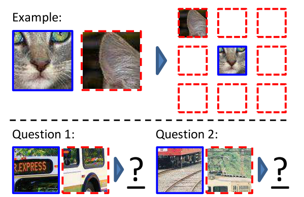
The algorithm receives two patches in one of these eight possible spatial arrangements without any context and must then classify which configuration was sampled.
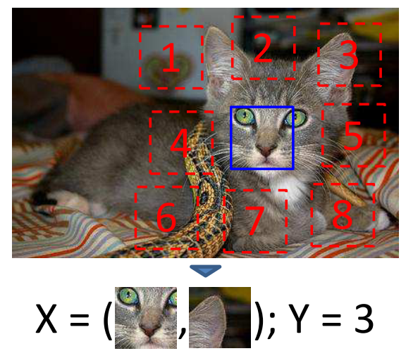
Centre-right: the location the trained network predicts for each patch shown on the left. Far-right: the same result after the colour projection scheme.

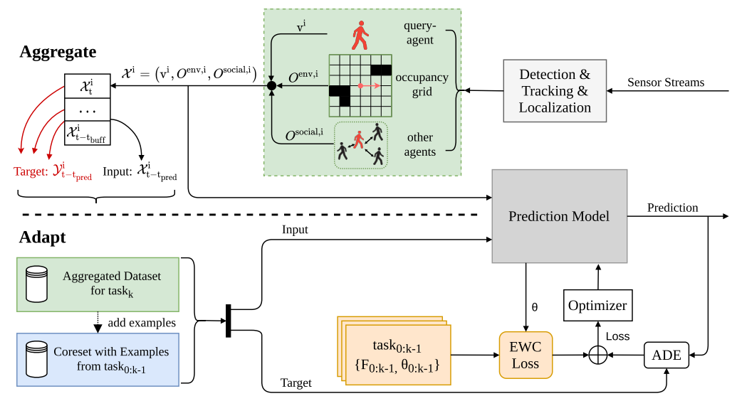
The following framework is extracting examples from the stream of tracked surrounding pedestrians.
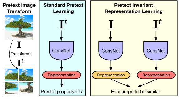
The representation must covary with the transformation $t$ and may not contain much semantic information. By contrast, pretext-invariant representation learning (PIRL) learns representations invariant to the transformation $t$ and retains semantic information.
Codes:
def model_fn(data, mode):
  """Produces a loss for the relative patch location task.
  Args:
    data: Dict of inputs ("image" being the image)
    mode: model's mode: training, eval or prediction
  Returns:
    EstimatorSpec
  """
  images = data['image']
  # Patch locations
  perms, num_classes = patch_utils.generate_patch_locations()
  labels = tf.tile(list(range(num_classes)), tf.shape(images)[:1])
  return patch_utils.creates_estimator_model(
      images, labels, perms, num_classes, mode)
Rotation
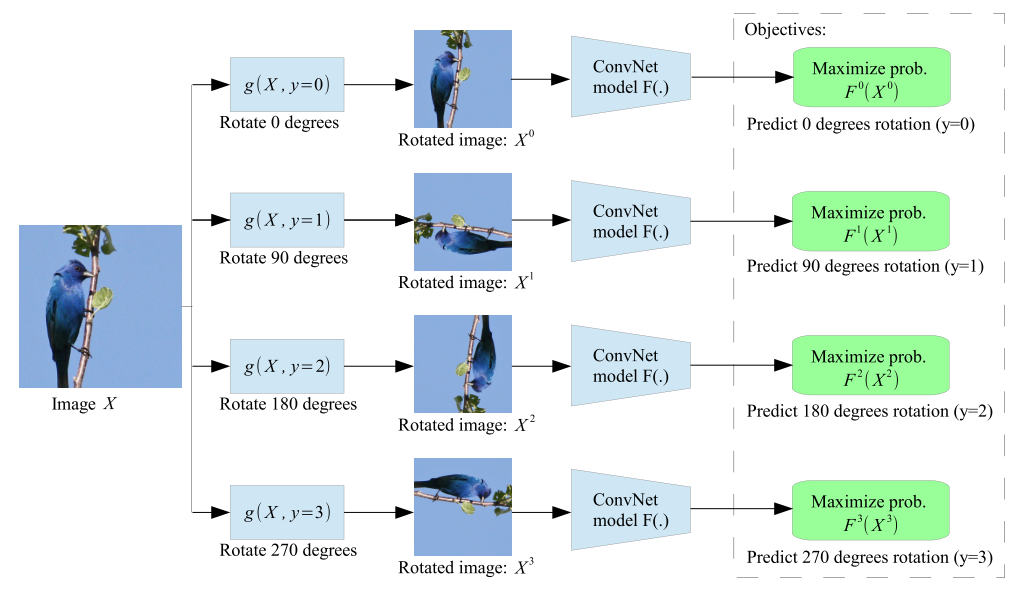
Training the ConvNets to recognise the geometric transformation applied to the image that it gets as input.
Given four possible geometric transformations, the 0, 90, 180, and 270 degrees rotations, we train a ConvNet model $F(.)$ to recognise the rotation applied to the image that it gets as input.

Codes:
Get rotation labels:
def get_iterator(self, epoch=0):
    rand_seed = epoch * self.epoch_size
    random.seed(rand_seed)
    if self.unsupervised:
        # if in unsupervised mode define a loader function that given the
        # index of an image it returns the 4 rotated copies of the image
        # plus the label of the rotation, i.e., 0 for 0 degrees rotation,
        # 1 for 90 degrees, 2 for 180 degrees, and 3 for 270 degrees.
        def _load_function(idx):
            idx = idx % len(self.dataset)
            img0, _ = self.dataset[idx]
            rotated_imgs = [
                self.transform(img0),
                self.transform(rotate_img(img0,  90)),
                self.transform(rotate_img(img0, 180)),
                self.transform(rotate_img(img0, 270))
            ]
            rotation_labels = torch.LongTensor([0, 1, 2, 3])
            return torch.stack(rotated_imgs, dim=0), rotation_labels
        def _collate_fun(batch):
            batch = default_collate(batch)
            assert(len(batch)==2)
            batch_size, rotations, channels, height, width = batch[0].size()
            batch[0] = batch[0].view([batch_size*rotations, channels, height, width])
            batch[1] = batch[1].view([batch_size*rotations])
            return batch
    else: # supervised mode
        # if in supervised mode define a loader function that given the
        # index of an image it returns the image and its categorical label
        def _load_function(idx):
            idx = idx % len(self.dataset)
            img, categorical_label = self.dataset[idx]
            img = self.transform(img)
            return img, categorical_label
        _collate_fun = default_collate
    tnt_dataset = tnt.dataset.ListDataset(elem_list=range(self.epoch_size),
        load=_load_function)
    data_loader = tnt_dataset.parallel(batch_size=self.batch_size,
        collate_fn=_collate_fun, num_workers=self.num_workers,
        shuffle=self.shuffle)
    return data_loader
Use unsupervised learning to train feature extractor (and classifier, not used in supervised training):
#********************************************************
start = time.time()
out_feat_keys = self.out_feat_keys
finetune_feat_extractor = self.optimizers['feat_extractor'] is not None
if do_train: # zero the gradients
    self.optimizers['classifier'].zero_grad()
    if finetune_feat_extractor:
        self.optimizers['feat_extractor'].zero_grad()
    else:
        self.networks['feat_extractor'].eval()
#********************************************************
#***************** SET TORCH VARIABLES ******************
dataX_var = Variable(dataX, volatile=((not do_train) or (not finetune_feat_extractor)))
labels_var = Variable(labels, requires_grad=False)
#********************************************************
#************ FORWARD PROPAGATION ***********************
feat_var = self.networks['feat_extractor'](dataX_var, out_feat_keys=out_feat_keys)
if not finetune_feat_extractor:
    if isinstance(feat_var, (list, tuple)):
        for i in range(len(feat_var)):
            feat_var[i] = Variable(feat_var[i].data, volatile=(not do_train))
    else:
        feat_var = Variable(feat_var.data, volatile=(not do_train))
pred_var = self.networks['classifier'](feat_var)
#********************************************************
#*************** COMPUTE LOSSES *************************
record = {}
if isinstance(pred_var, (list, tuple)):
    loss_total = None
    for i in range(len(pred_var)):
        loss_this = self.criterions['loss'](pred_var[i], labels_var)
        loss_total = loss_this if (loss_total is None) else (loss_total + loss_this)
        record['prec1_c'+str(1+i)] = accuracy(pred_var[i].data, labels, topk=(1,))[0][0]
        record['prec5_c'+str(1+i)] = accuracy(pred_var[i].data, labels, topk=(5,))[0][0]
else:
    loss_total = self.criterions['loss'](pred_var, labels_var)
    record['prec1'] = accuracy(pred_var.data, labels, topk=(1,))[0][0]
    record['prec5'] = accuracy(pred_var.data, labels, topk=(5,))[0][0]
record['loss'] = loss_total.data[0]
#********************************************************
#****** BACKPROPAGATE AND APPLY OPTIMIZATION STEP *******
if do_train:
    loss_total.backward()
    self.optimizers['classifier'].step()
    if finetune_feat_extractor:
        self.optimizers['feat_extractor'].step()
#********************************************************
Use supervised learning to train classifier:
self.tensors['dataX'].resize_(batch[0].size()).copy_(batch[0])
self.tensors['labels'].resize_(batch[1].size()).copy_(batch[1])
dataX = self.tensors['dataX']
labels = self.tensors['labels']
batch_load_time = time.time() - start
#********************************************************
#********************************************************
start = time.time()
if do_train: # zero the gradients
    self.optimizers['model'].zero_grad()
#********************************************************
#***************** SET TORCH VARIABLES ******************
dataX_var = torch.autograd.Variable(dataX, volatile=(not do_train))
labels_var = torch.autograd.Variable(labels, requires_grad=False)
#********************************************************
#************ FORWARD THROUGH NET ***********************
pred_var = self.networks['model'](dataX_var)
#********************************************************
#*************** COMPUTE LOSSES *************************
record = {}
loss_total = self.criterions['loss'](pred_var, labels_var)
record['prec1'] = accuracy(pred_var.data, labels, topk=(1,))[0][0]
record['loss'] = loss_total.data[0]
#********************************************************
#****** BACKPROPAGATE AND APPLY OPTIMIZATION STEP *******
if do_train:
    loss_total.backward()
    self.optimizers['model'].step()
#********************************************************
batch_process_time = time.time() - start
total_time = batch_process_time + batch_load_time
record['load_time'] = 100*(batch_load_time/total_time)
record['process_time'] = 100*(batch_process_time/total_time)
In unsupervised learning, the feature extractor and classifier are trained. Use rotation degree labels.
data_test_opt['unsupervised'] = TrueIn supervised learning, only the classifier is trained. But feature extractor is from unsupervised learning.
data_test_opt['unsupervised'] = FalseJigsaw
The task is to recover the spatial position of 9 randomly sampled image patches. Learning image representations is achieved by completing damaged jigsaw puzzles.
To avoid shortcuts relying on low-level image statistics such as chromatic aberration or edge alignment, patches are sampled with a random gap between them. Chromatic aberration, also known as colour fringing, is a colour distortion that creates an outline of unwanted colour along the edges of objects in a photograph.
Left image: the puzzles after shuffling the patches, removing one patch, and decolourising. A network was proposed to recover the original arrangement, the missing patch, and the colour of the puzzles.
Right image: The output.
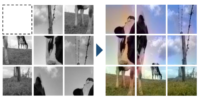
The architecture for “completing damaged jigsaw puzzles”. Blue, red, and orange represent jigsaw puzzles, inpainting, and colourisation, respectively.

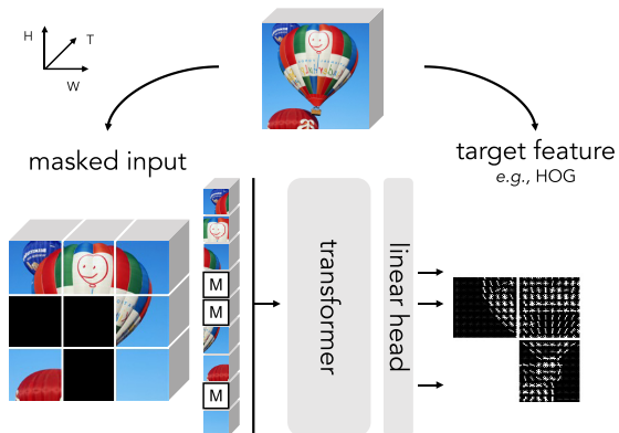
Histograms of Oriented Gradients (HOG) is learned by predicting features (middle) given masked input (left).
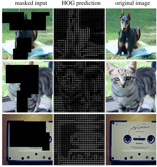
Input space-time cubes of a video with a [MASK] token and directly regress the masked regions’ features (e.g., HOG). After pre-training, the Transformer is fined-tuned on end tasks.
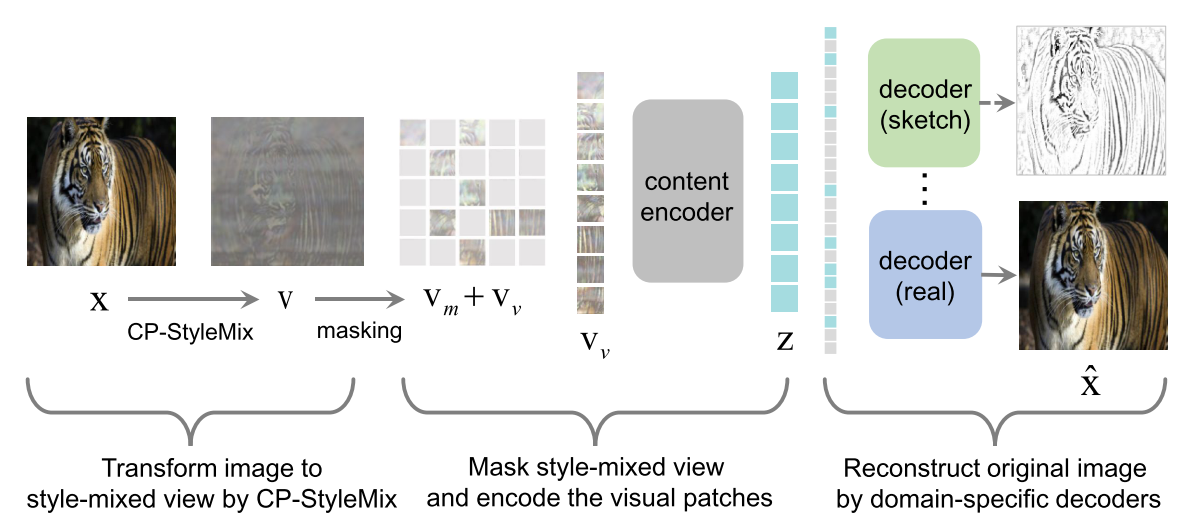
Domain-specific decoders learn to reconstruct $\hat{x}$ by the corresponding decoder.
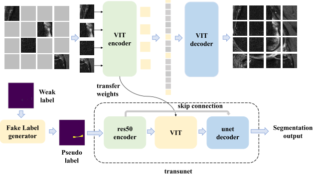
Use ViT as the framework’s encoder and decoder.
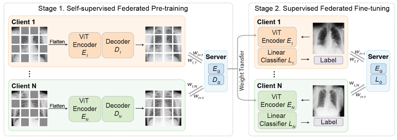
Self-supervised technique in federated learning.
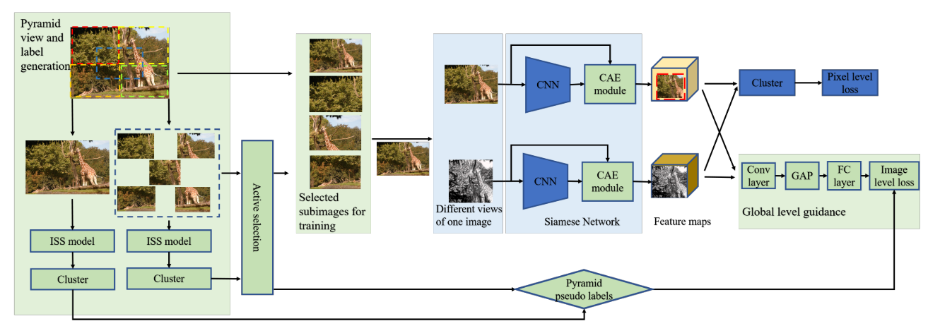
The whole framework is guided by the pyramid global guidance (PGG) strategy, including the pyramid view and label generation, active selection, and the global-level guidance in the clustering process.
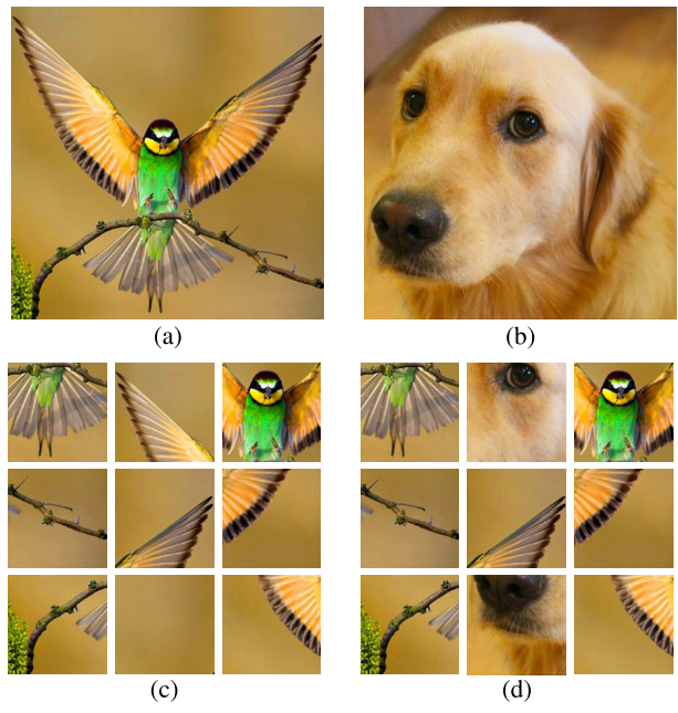
In the following image,
(c) Jigsaw: 9 randomly sampled image patches after a random permutation of these patches was performed.
(d) Jigsaw++: At most, 2 tiles can come from a random image.
Codes:
def model_fn(data, mode):
  """Produces a loss for the jigsaw task.
  Args:
    data: Dict of inputs ("image" being the image)
    mode: model's mode: training, eval or prediction
  Returns:
    EstimatorSpec
  """
  images = data['image']
  # Patch locations
  perms, num_classes = patch_utils.load_permutations()
  labels = list(range(num_classes))
  # Selects a subset of permutation for training. There're two methods:
  #   1. For each image, selects 16 permutations independently.
  #   2. For each batch of images, selects the same 16 permutations.
  # Here we used method 2, for simplicity.
  if mode in [tf.estimator.ModeKeys.TRAIN]:
    perm_subset_size = FLAGS.get_flag_value('perm_subset_size', 8)
    indexs = list(range(num_classes))
    indexs = tf.random_shuffle(indexs)
    labels = indexs[:perm_subset_size]
    perms = tf.gather(perms, labels, axis=0)
    tf.logging.info('subsample %s' % perms)
  labels = tf.tile(labels, tf.shape(images)[:1])
  return patch_utils.creates_estimator_model(
      images, labels, perms, num_classes, mode)
Exemplar
Every individual image corresponds to its own class, and multiple examples of it are generated by heavy random data augmentation such as translation, scaling, rotation, contrast, and colour shifts. Alexander et al. used triplet loss to avoid explicit class labels. Instead, it encourages examples of the same image to have representations close in the Euclidean space while also being far from the representations of different images.
Left: Exemplary patches sampled from the unlabelled dataset.
Right: Several random transformations were applied to one of the patches extracted from the unlabelled dataset.

Use patch count as label and get triplets loss. Part codes:
labels = repeat(tf.range(batch_size), patch_count)
norm_logits = tf.nn.l2_normalize(logits, axis=0)
loss = tf.contrib.losses.metric_learning.triplet_semihard_loss(
    labels, norm_logits, margin=FLAGS.margin)
return make_estimator(mode, loss, predictions=logits)
Contrastive learning
Contrastive analysis is the sytematic study of a pair of lanaugaes with a view to identifying their structureal differences and similarities.
Training data can be divided into positive examples and negative examples. Positive examples are those that match the target. For example, if your’re learning to identify birds, the positive training data are those pictures that contains birds. Negative examples are those that do not match the target.
Contrastive self-supervised leanring
Contrastive self-supervised learning (SSL) uses both positive and negative examples. Contrastive learning’s loss function minimises the distance between positive samples while maximising the distance between negative samples.
SimCLR
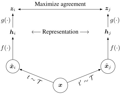
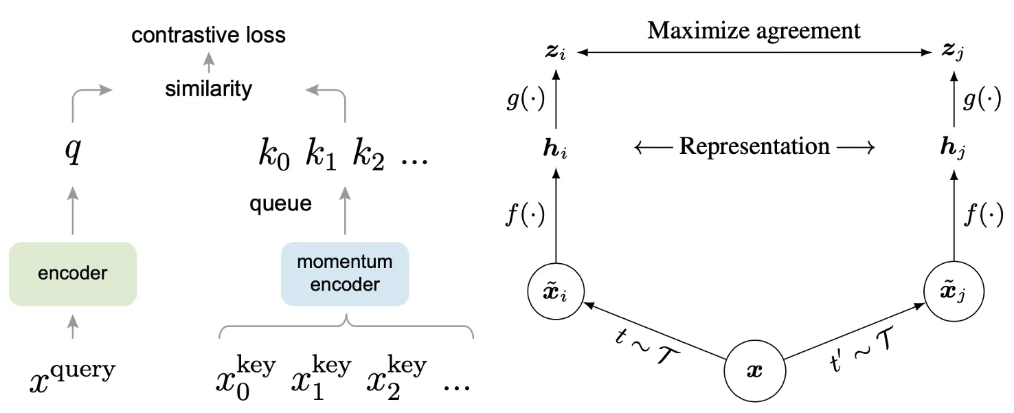
A simple framework for contrastive learning of visual representations (SimCLR). Two separate data augmentation operators are sampled from the same family of augmentations ($t ~ \mathcal{T}$ and $t ^ {‘} ~ \mathcal{T}$) and applied to each data example to obtain two correlated views. A base encodes network $f(.)$, and a projection head $g(.)$ are trained to maximise agreement using a contrastive loss.
After training is completed, the projection head $g(.)$ is thrown away, and the encoder $f(.)$ and representation $h$ are utilised for downstream tasks.
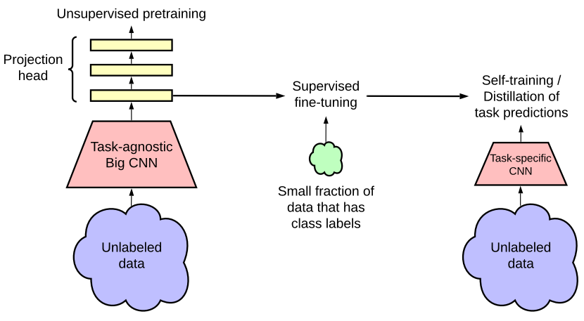
This semi-supervised learning framework leverages unlabelled data: (1) task-agnostic use in unsupervised pre-training and (2) task-specific use in self-training/ distillation.
The fewer the labels, the more task agnostic use of unlabelled data benefits from a more extensive network (deeper and broader).
MoCo vs SimCLR
The way of generating the key representations in these two approaches are different. In MoCo, the key (momentum) encoder is separated from the query encoder, they have identical architecture, and the parameters of the key encoder are updated by the parameters of the query encoder.
By contrast, there is only one encoder in SimCLR which is used for the generation of both query and key representations.
Others
Self-supervised video representation learning
Design different pretext tasks: speed perception, order prediction, temporal transformation, order prediction, motion estimation, temporal transformation discrimination, object consistency, and future prediction.
Apply constrastive learning: Image paradigm, spatio-temporal transformations for videos.
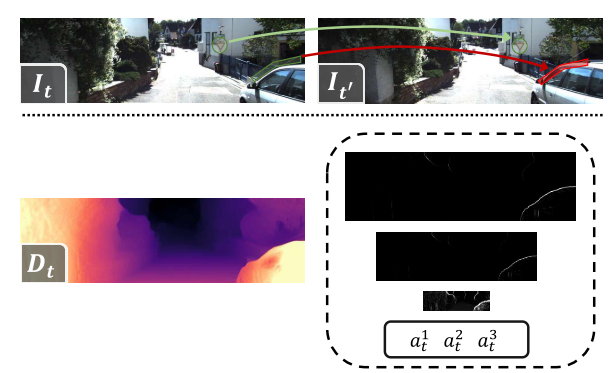
e.g., A guided filtering-based method is used to find these potentially occluded areas.
NTXent and InfoNCE
NT-Xent excludes the positive sample from the denominator whereas InfoNCE includes it. In the papers there is some variation in how they get the embeddings and which (combination of) samples they use for the loss, but functionally it essentially comes down to doing softmax on embeddings.
Consine similarity
Given two vectors $a$ and $b$, the angle $θ$ is obtained by the scalar product and the norm of the vectors:
$$ cos(\theta) = \frac{a \cdot b}{||a|| \cdot ||b||} $$
Since $-1 \leq cos(\theta) \leq 1$,
- $-1$ indicates strongly opposite vectors
- $0$ independent (orthogonal) vectors
- $1$ similar (positive co-linear) vectors. Intermediate values are
used to assess the degree of similarity.
Example : Let two users $U_1$ and $U_2$, and $sim(U_1, U_2)$ be the similarity between these two users according to their taste for movies:
- $sim(U_1, U_2) = 1$ if the two users have exactly the same taste (or if $U_1 = U_2$)
- $sim(U_1, U_2) = 0$ if we do not find any correlation between the two users, e.g. if they have not seen any common movies
- $sim(U_1, U_2) = -1$ if users have opposed tastes, e.g. if they rated the same movies in an opposite way
Reference
[1] Zhai, X., Oliver, A., Kolesnikov, A. and Beyer, L., 2019. S4l: Self-supervised semi-supervised learning. In Proceedings of the IEEE/CVF International Conference on Computer Vision (pp. 1476-1485).
[2] Kolesnikov, A., Zhai, X. and Beyer, L., 2019. Revisiting self-supervised visual representation learning. In Proceedings of the IEEE/CVF conference on computer vision and pattern recognition (pp. 1920-1929).
[3] Doersch, C., Gupta, A. and Efros, A.A., 2015. Unsupervised visual representation learning by context prediction. In Proceedings of the IEEE international conference on computer vision (pp. 1422-1430).
[4] Knoedler, L., Salmi, C., Zhu, H., Brito, B. and Alonso-Mora, J., 2022. Improving Pedestrian Prediction Models with Self-Supervised Continual Learning. IEEE Robotics and Automation Letters, 7(2), pp.4781-4788.
[5] Misra, I. and Maaten, L.V.D., 2020. Self-supervised learning of pretext-invariant representations. In Proceedings of the IEEE/CVF Conference on Computer Vision and Pattern Recognition (pp. 6707-6717).
[6] Gidaris, S., Singh, P. and Komodakis, N., 2018. Unsupervised representation learning by predicting image rotations. arXiv preprint arXiv:1803.07728.
[7] gidariss/FeatureLearningRotNet
[8] Dosovitskiy, A., Springenberg, J.T., Riedmiller, M. and Brox, T., 2014. Discriminative unsupervised feature learning with convolutional neural networks. Advances in neural information processing systems, 27.
[9] google/revisiting-self-supervised
[10] Kim, D., Cho, D., Yoo, D. and Kweon, I.S., 2018, March. Learning image representations by completing damaged jigsaw puzzles. In 2018 IEEE Winter Conference on Applications of Computer Vision (WACV) (pp. 793-802). IEEE.
[11] Wei, C., Fan, H., Xie, S., Wu, C.Y., Yuille, A. and Feichtenhofer, C., 2021. Masked Feature Prediction for Self-Supervised Visual Pre-Training. arXiv preprint arXiv:2112.09133.
[12] Yang, H., Chen, M., Wang, Y., Tang, S., Zhu, F., Bai, L., Zhao, R. and Ouyang, W., 2022. Domain Invariant Masked Autoencoders for Self-supervised Learning from Multi-domains. arXiv preprint arXiv:2205.04771.
[13] Xie, Y., Jiang, K., Zhang, Z., Chen, S., Zhang, X. and Qiu, C., 2022. Automatic segmentation of meniscus based on MAE self-supervision and point-line weak supervision paradigm. arXiv preprint arXiv:2205.03525.
[14] Yan, R., Qu, L., Wei, Q., Huang, S.C., Shen, L., Rubin, D., Xing, L. and Zhou, Y., 2022. Label-Efficient Self-Supervised Federated Learning for Tackling Data Heterogeneity in Medical Imaging. arXiv preprint arXiv:2205.08576.
[15] Wang, Y., Zhuo, W., Li, Y., Wang, Z., Ju, Q. and Zhu, W., 2022. Fully Self-Supervised Learning for Semantic Segmentation. arXiv preprint arXiv:2202.11981.
[16] Noroozi, M., Vinjimoor, A., Favaro, P. and Pirsiavash, H., 2018. Boosting self-supervised learning via knowledge transfer. In Proceedings of the IEEE Conference on Computer Vision and Pattern Recognition (pp. 9359-9367).
[17] Chen, T., Kornblith, S., Norouzi, M. and Hinton, G., 2020, November. A simple framework for contrastive learning of visual representations. In International conference on machine learning (pp. 1597-1607). PMLR.
[18] Chen, T., Kornblith, S., Swersky, K., Norouzi, M. and Hinton, G.E., 2020. Big self-supervised models are strong semi-supervised learners. Advances in neural information processing systems, 33, pp.22243-22255.
[19] Qing, Z., Zhang, S., Huang, Z., Xu, Y., Wang, X., Tang, M., Gao, C., Jin, R. and Sang, N., 2022. Learning from Untrimmed Videos: Self-Supervised Video Representation Learning with Hierarchical Consistency. arXiv preprint arXiv:2204.03017.
[20] Yang, X., Zhang, S. and Zhao, B., 2021, July. Self-Supervised Monocular Depth Estimation with Multi-constraints. In 2021 40th Chinese Control Conference (CCC) (pp. 8422-8427). IEEE.
[22] Contrastive Learning: Comparison Between Architectures of MoCo and SimCLR.
本博客所有文章除特别声明外,均采用 CC BY-SA 4.0 协议 ,转载请注明出处!