Last updated on：a year ago

Semi-supervised learning is a learning paradigm concerned with how to learn the presence of both labelled and unlabelled data.

Introduction

Semi-supervised learning is an approach to machine learning that combines a small amount of labelled data with many unlabelled data during training. It falls between unsupervised learning and supervised learning.

Motivation

Unlabelled data is easy to be obtained.
Labelled data can be hard to get.
Labelled data sometimes is scarce or expensive.

Semi-supervised learning is of great interest in machine learning and data mining because it can use readily available unlabelled data to improve supervised learning tasks.

Goal

Semi-supervised learning mixes labelled and unlabelled data to produce better models.

Semi-supervised learning aims to understand how combining labelled, and unlabelled data may change the learning behaviour, and design algorithms that take advantage of such a combination.

Two distinct goals: (a) predict the labels on future test data **(inductive semi-supervised learning). (b) predict the labels on the unlabelled instances in the training example **(transductive learning).

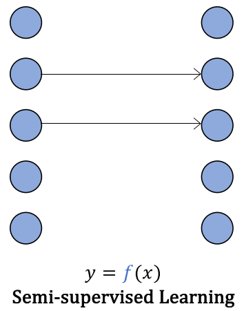
The data point of view

Data in both input $x$ and output $y$ with known partial mapping (learn the mapping $f$)

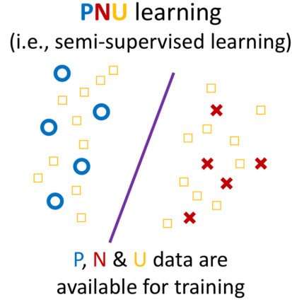
PNU learning. P: positive data, N: negative data, U: unlabelled data

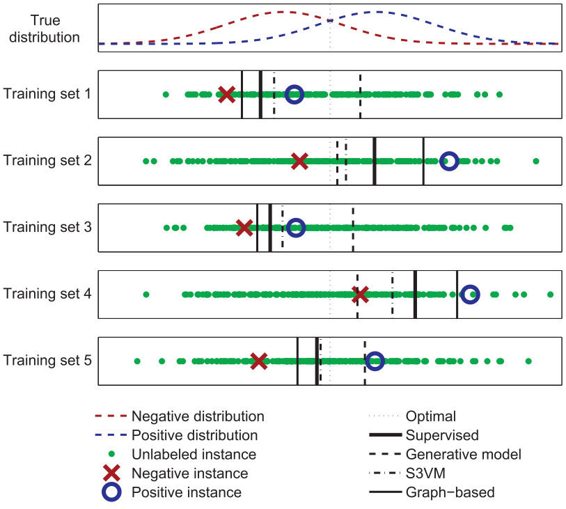
How does semi-supervised learning work?

Instances in each class form a coherent group (e.g., $p(\bf{x}|y)$) is a Gaussian distribution, such that the instances from each class centre around a central mean. The distribution of unlabelled data helps identify regions with the same label, and the few labelled data then provide the actual labels.

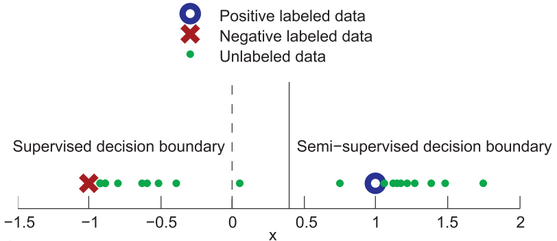
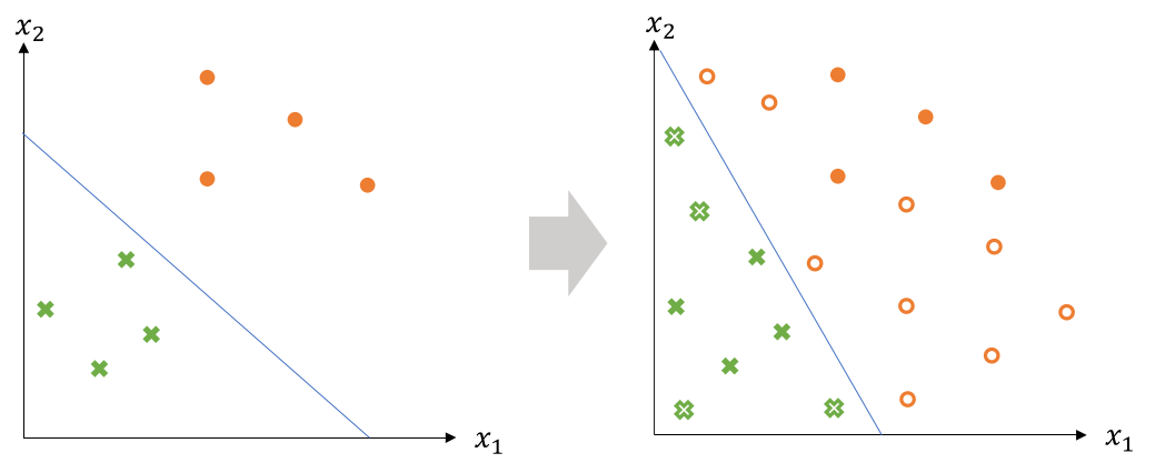
Unlabelled data can help to find a better boundary.

Semi-supervised Learning Methods

Semi-supervised learning is of great interest in machine learning and data mining because it can use readily available unlabelled data to improve supervised learning tasks.

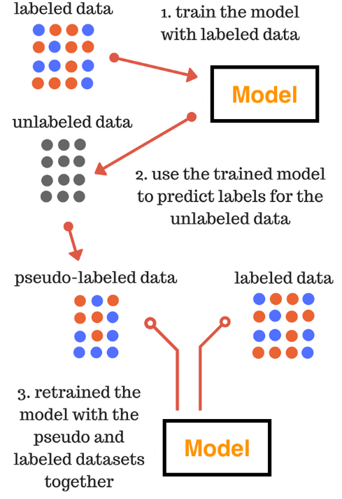
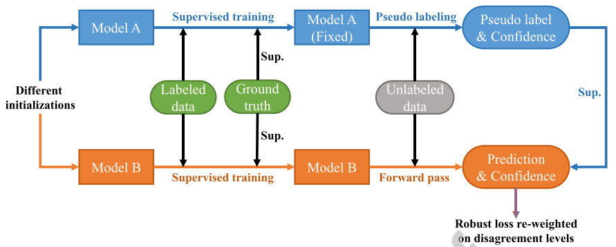
Pseudo Labelling

Pseudo means not genuine, spurious or sham.

Pseudo labelling is adding confidently predicted test data to our training data. Pseudo labelling is a 5 step process:

(1) Build a model using training data.

(2) Predict labels for an unseen test dataset.

(3) Add confidently predicted test observations to our training data.

(4) Build a new model using combined data.

(5) Use your new model to predict the test data.

Self-training

Pseudo labelling is widely used in self-training. Self-training is one of the most used semi-supervised methods.

Self-training algorithms is to learn a classifier iteratively by assigning pseudo-labels to the set of unlabelled training samples with a margin greater than a certain threshold. The pseudo-labelled examples are then used to enrich the labelled training data and train a new classifier in conjunction with the labelled training set.

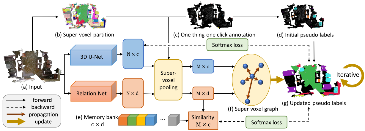
Liu et al. used one point on a subject to generate the initial pseudo labels. They use a super-voxel graph to propagate labels over the point cloud to further iteratively update the predicted labels.

Application

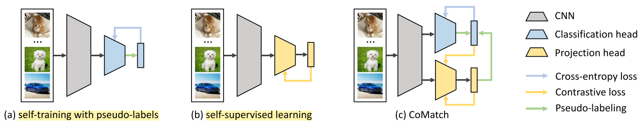
Classification

Task-specific self-training: the model predicts class probabilities for the unlabelled samples as the pseudo-label to train again.

Task-agnostic self-supervised training: the model projects samples into low-dimensional embeddings and performs contrastive learning to discriminate embeddings of different images.

CoMatch: class probabilities and embeddings interact and jointly evolve in a co-training framework. The embedding imposes a smoothness constraint on the class probabilities to improve the pseudo-labels.

Codes:

Training:

ims_x_weak, lbs_x = next(dl_x)
(ims_u_weak, ims_u_strong0, ims_u_strong1), lbs_u_real = next(dl_u)
lbs_x = lbs_x.cuda()
lbs_u_real = lbs_u_real.cuda()
# --------------------------------------
bt = ims_x_weak.size(0)
btu = ims_u_weak.size(0)
imgs = torch.cat([ims_x_weak, ims_u_weak, ims_u_strong0, ims_u_strong1], dim=0).cuda()
logits, features = model(imgs)
logits_x = logits[:bt]
logits_u_w, logits_u_s0, logits_u_s1 = torch.split(logits[bt:], btu)
feats_x = features[:bt]
feats_u_w, feats_u_s0, feats_u_s1 = torch.split(features[bt:], btu)
loss_x = criteria_x(logits_x, lbs_x)

with torch.no_grad():
    logits_u_w = logits_u_w.detach()
    feats_x = feats_x.detach()
    feats_u_w = feats_u_w.detach()
    
    probs = torch.softmax(logits_u_w, dim=1)            
    # DA
    prob_list.append(probs.mean(0))
    if len(prob_list)>32:
        prob_list.pop(0)
    prob_avg = torch.stack(prob_list,dim=0).mean(0)
    probs = probs / prob_avg
    probs = probs / probs.sum(dim=1, keepdim=True)   
    probs_orig = probs.clone()
    
    if epoch>0 or it>args.queue_batch: # memory-smoothing 
        A = torch.exp(torch.mm(feats_u_w, queue_feats.t())/args.temperature)       
        A = A/A.sum(1,keepdim=True)                    
        probs = args.alpha*probs + (1-args.alpha)*torch.mm(A, queue_probs)               
    
    scores, lbs_u_guess = torch.max(probs, dim=1)
    mask = scores.ge(args.thr).float() 
            
    feats_w = torch.cat([feats_u_w,feats_x],dim=0)   
    onehot = torch.zeros(bt,args.n_classes).cuda().scatter(1,lbs_x.view(-1,1),1)
    probs_w = torch.cat([probs_orig,onehot],dim=0)
    
    # update memory bank
    n = bt+btu   
    queue_feats[queue_ptr:queue_ptr + n,:] = feats_w
    queue_probs[queue_ptr:queue_ptr + n,:] = probs_w      
    queue_ptr = (queue_ptr+n)%args.queue_size

Embedding similarity;

sim = torch.exp(torch.mm(feats_u_s0, feats_u_s1.t())/args.temperature) 
sim_probs = sim / sim.sum(1, keepdim=True)

Contrastive loss:

loss_contrast = - (torch.log(sim_probs + 1e-7) * Q).sum(1)
loss_contrast = loss_contrast.mean()

Unsupervised classification loss:

loss_u = - torch.sum((F.log_softmax(logits_u_s0,dim=1) * probs),dim=1) * mask                
loss_u = loss_u.mean()
loss = loss_x + args.lam_u * loss_u + args.lam_c * loss_contrast

Pseudo-label graph with self-loop:

Q = torch.mm(probs, probs.t())       
Q.fill_diagonal_(1)    
pos_mask = (Q>=args.contrast_th).float()
Q = Q * pos_mask
Q = Q / Q.sum(1, keepdim=True)

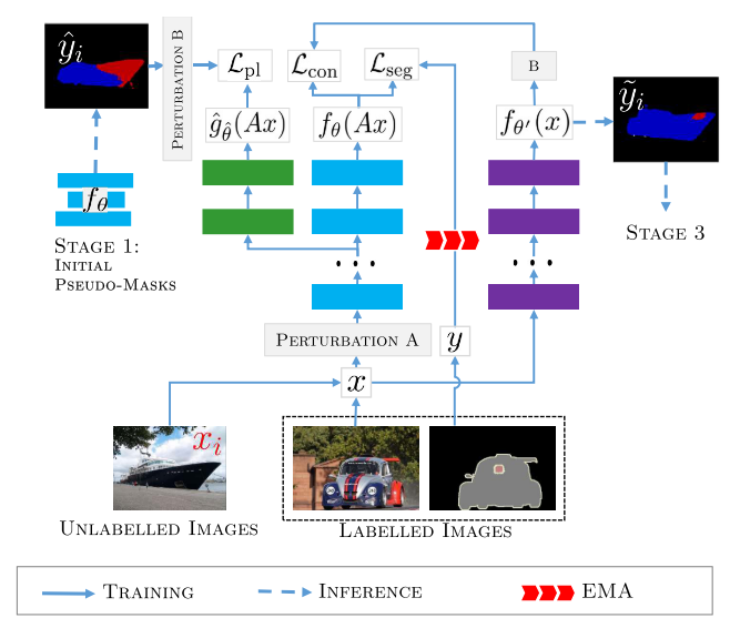
pos_meter.update(pos_mask.sum(1).float().mean().item())

Segmentation

There are two different models trained on the labelled subset, and one model provides pseudo supervisions for the other.

Ke et al. generate a pseudo mask for unlabelled data while enforcing segmentation consistency in a multi-task fashion. (rough masks - > higher quality masks)

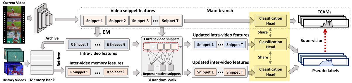
Localization

The peripheral branch is first trained in the warm-up epoches. After that, the peripheral branch supervises main branch by its loss and output label.

Codes:

for num, sample in enumerate(self.train_data_loader):
    if self.args.decay_type == 0:
        for param_group in self.optimizer_module.param_groups:
            param_group['lr'] = current_lr
    elif self.args.decay_type == 1:
        if num == 0:
            current_lr = self.Step_decay_lr(epoch)
            for param_group in self.optimizer_module.param_groups:
                param_group['lr'] = current_lr
    elif self.args.decay_type == 2:
        current_lr = self.Cosine_decay_lr(epoch, num)
        for param_group in self.optimizer_module.param_groups:
            param_group['lr'] = current_lr
    iter = iter + 1
    np_features = sample['data'].numpy()
    np_labels = sample['labels'].numpy()
    labels = torch.from_numpy(np_labels).float().to(self.device)
    features = torch.from_numpy(np_features).float().to(self.device)
    f_labels = torch.cat([labels, torch.zeros(labels.size(0), 1).to(self.device)], -1)
    b_labels = torch.cat([labels, torch.ones(labels.size(0), 1).to(self.device)], -1)
    # the output and loss of peripheral branch will be used to supervise main branch
    o_out, m_out, em_out = self.model(features)
    vid_fore_loss = self.loss_nce(o_out[0], f_labels) + self.loss_nce(m_out[0], f_labels)
    vid_back_loss = self.loss_nce(o_out[1], b_labels) + self.loss_nce(m_out[1], b_labels)
    vid_att_loss = self.loss_att(o_out[2])
    # use warm-up epoch only in peripheral branch
    if epoch > self.args.warmup_epoch:
        idxs = np.where(np_labels==1)[0].tolist()
        cls_mu = self.memory._return_queue(idxs).detach()
        reallocated_x = random_walk(em_out[0], cls_mu, self.args.w)
        r_vid_ca_pred, r_vid_cw_pred, r_frm_fore_att, r_frm_pred = self.model.PredictionModule(reallocated_x)
        vid_fore_loss += 0.5 * self.loss_nce(r_vid_ca_pred, f_labels)
        vid_back_loss += 0.5 * self.loss_nce(r_vid_cw_pred, b_labels)
        vid_spl_loss = self.loss_spl(o_out[3], r_frm_pred * 0.2 + m_out[3] * 0.8)
        self.memory._update_queue(em_out[1].squeeze(0), em_out[2].squeeze(0), idxs)
    else:
        vid_spl_loss = self.loss_spl(o_out[3], m_out[3])
    total_loss = vid_fore_loss + vid_back_loss * self.args.lambda_b \
    + vid_att_loss * self.args.lambda_a + vid_spl_loss * self.args.lambda_s
    loss_recorder['cls_fore'] += vid_fore_loss.item()
    loss_recorder['cls_back'] += vid_back_loss.item()
    loss_recorder['att'] += vid_att_loss.item()
    loss_recorder['spl'] += vid_spl_loss.item()
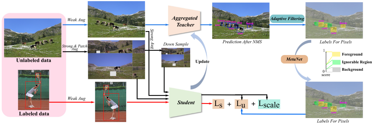
    total_loss.backward()

Detection

A teacher model is employed during each training iteration to produce pseudo-labels for weakly augmented unlabelled images.

Generative methods (GE)

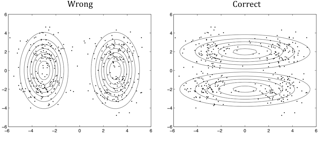
Unlabelled data shows how the instances from all the mixed together classes, are distributed.

EM with some labelled data: cluster and then label.

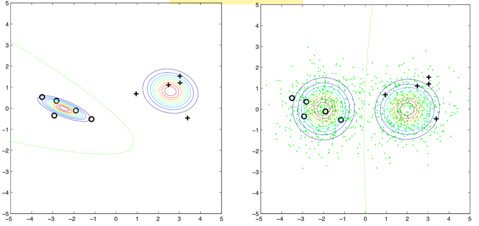
Unlabelled data may hurt the learning.

Graph-based methods

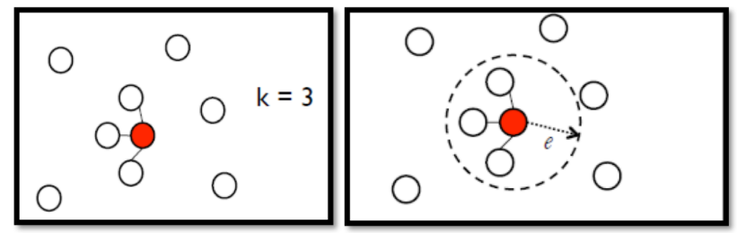
(1) Define the similarity $s(x_i, x_j)$

(2) Add edges: KNN, e-Neighbourhood

(3) Edge weight is proportional to $s(x_i, x_j)$

(4) Propagate through the graph

Reference

[1] Zhu, X. and Goldberg, A.B., 2009. Introduction to semi-supervised learning. Synthesis lectures on artificial intelligence and machine learning, 3(1), pp.1-130.

[2] Wiki, Semi-supervised learning.

[3] Hao Dong, Learning Methods.

[4] Kaggle, Pseudo Labelling.

[5] Chen, B., Li, P., Chen, X., Wang, B., Zhang, L. and Hua, X.S., 2022. Dense Learning based Semi-Supervised Object Detection. arXiv preprint arXiv:2204.07300.

[6] Li, J., Xiong, C. and Hoi, S.C., 2021. Comatch: Semi-supervised learning with contrastive graph regularization. In Proceedings of the IEEE/CVF International Conference on Computer Vision (pp. 9475-9484).

[7] salesforce/CoMatch

[8] Amini, M.R., Feofanov, V., Pauletto, L., Devijver, E. and Maximov, Y., 2022. Self-Training: A Survey. arXiv preprint arXiv:2202.12040.

[9] Huang, L., Wang, L. and Li, H., 2022. Weakly Supervised Temporal Action Localization via Representative Snippet Knowledge Propagation. arXiv preprint arXiv:2203.02925.

[10] LeonHLJ/RSKP

Deep learning Machine learning

semi-supervised

本博客所有文章除特别声明外，均采用 CC BY-SA 4.0 协议，转载请注明出处！

One server can collaborate with global clients using federated learning Previous

Let's register images to demonstrate their features Next

Semi-supervised learning and its goal