Spiking neural networks are bio-inspired artificial intelligence method to process signal efficiently with low power consumpsion binary signal mechanism.

Introduction

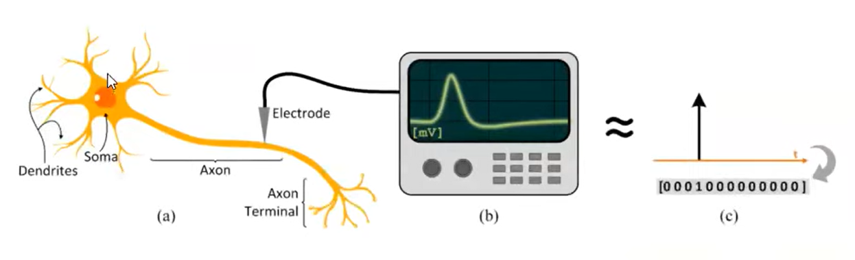
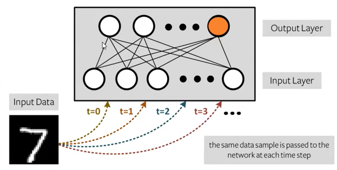
Spiking neural networks (SNNs) are ANNs that more closely mimic natural neural networks. Neurons only transmit data when their “membrane potential” reaches a threshold. Transmitted spikes will either increase or decrease the membrane potentials of other neurons. SNNs utilise the concept of time in their execution.

Spiking neural networks (SNNs) are artificial neural networks (ANNs) that more closely mimic natural neural networks. In addition to neuronal and synaptic states, SNNs incorporate the concept of time into their operating model.

Spiking neural networks offer an alternative for enabling energy-efficient intelligence, which emulates biological neuronal functionality by adopting binary spiking signals to complete inter-neuron communication.

Motivation

SNN characteristics

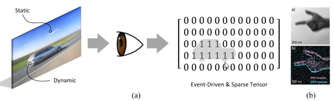
• Spikes: biological neurons interact via single-bite spikes. We only care about whether the action potential occurs.
  
• Sparsity: biological neurons spend most of their time at rest, setting most activations to zero at any given time.
• Static suppression (aka event-driven processing). The sensory periphery only processes information when there is new information to process.
  

SNN advantages

• Energy efficiency
• Area efficiency (does not inherently feature any large scale matrix multiplication), needs only adders and comparators.
• Efficient On-Chip learning
• Fault tolerance
• Training very deep networks is made super simple

Problems

• SNN is an approximation of the ANN
• Temporal ANN conversion is underexplored
• Biologically implausible
  For native SNN training:
• Less efficient on modern hardware
• Very sensitive to hyperparameters

Encoding data for SNNs

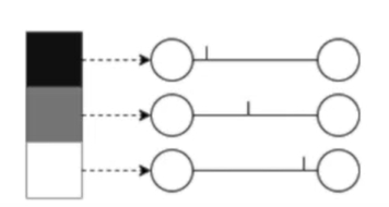
Rate coding: the neurons corresponding to inputs with the highest intensities fire more frequently. Information is stored in the spike count or firing rate.

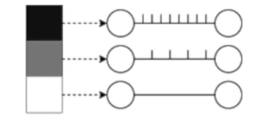
Temporal coding: the neurons corresponding to inputs with the highest intensities fire first. Information is stored at the time of a spike.
Rates are better for error and noise tolerance and enable faster convergence when using backprop. Timing is better for power efficiency and latency.

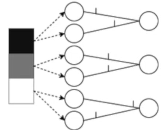
Population coding: the spike times of several input neurons are used to represent the input data.

Neural models for SNNs

Integrate and fire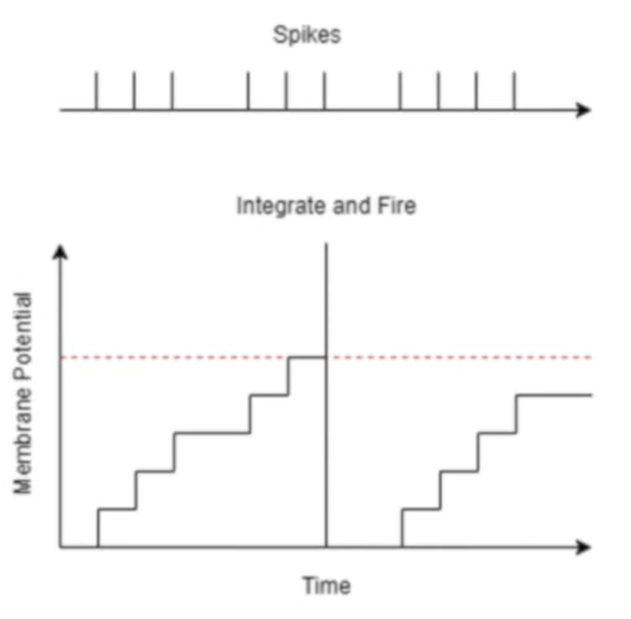

Leaky integrate and fire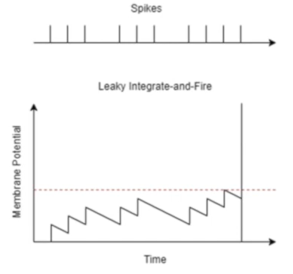

Adaptive leaky integrate and fire
Prevent it from firing quickly again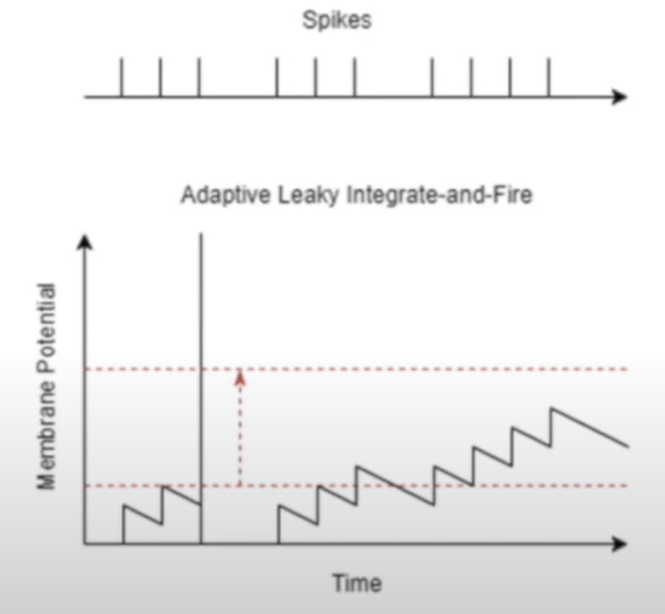

Learning techniques for SNNs

Spike-timing-dependent-plasticity (STDP)
Weight is increased if the pre-synaptic neuron fires just before the post-synaptic neuron.
Also known as long-term potentiation (LTP)
Weight is increased if the post-synaptic neuron fires just before the post-synaptic neuron
Also known as long-term depression (LTD)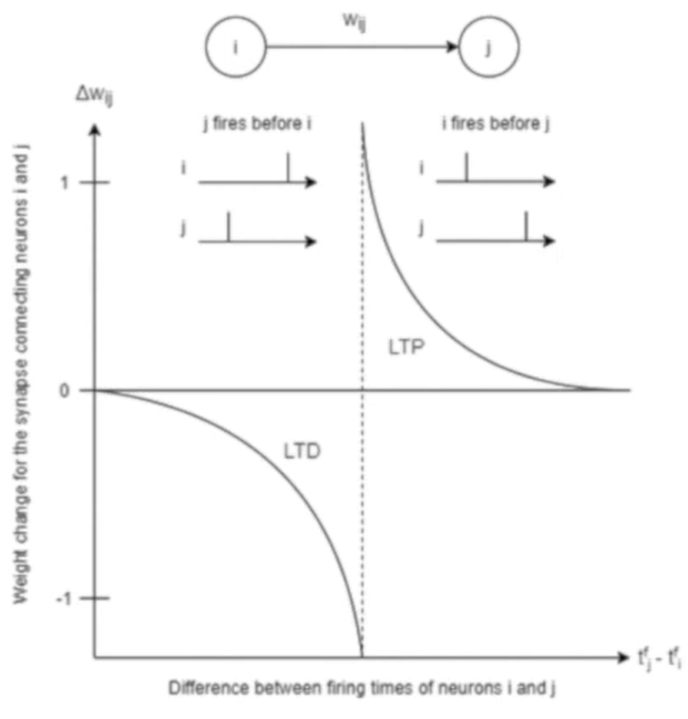

Challenges with implementing SNNs

• Training is difficult
• Accuracy does not match that of traditional ANNs
• Need better metrics to benchmark SNN performance relative to ANNs
• Programming frameworks are still in their infancy

Potential areas of improvement

• Modify the learning rate based on the batch size
• Use a smaller batch size to improve training accuracy
• Increase the neuron count in the excitatory layer
• Increase the number of simulation timesteps to improve accuracy
• Increase the number of epochs (training samples) to improve accuracy
• Adjust the hyperparameters to accommodate the variations in encoding schemes, neural models and learning techniques

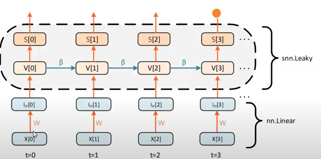
Leaky integrate-and-fire neuron

Generate spike: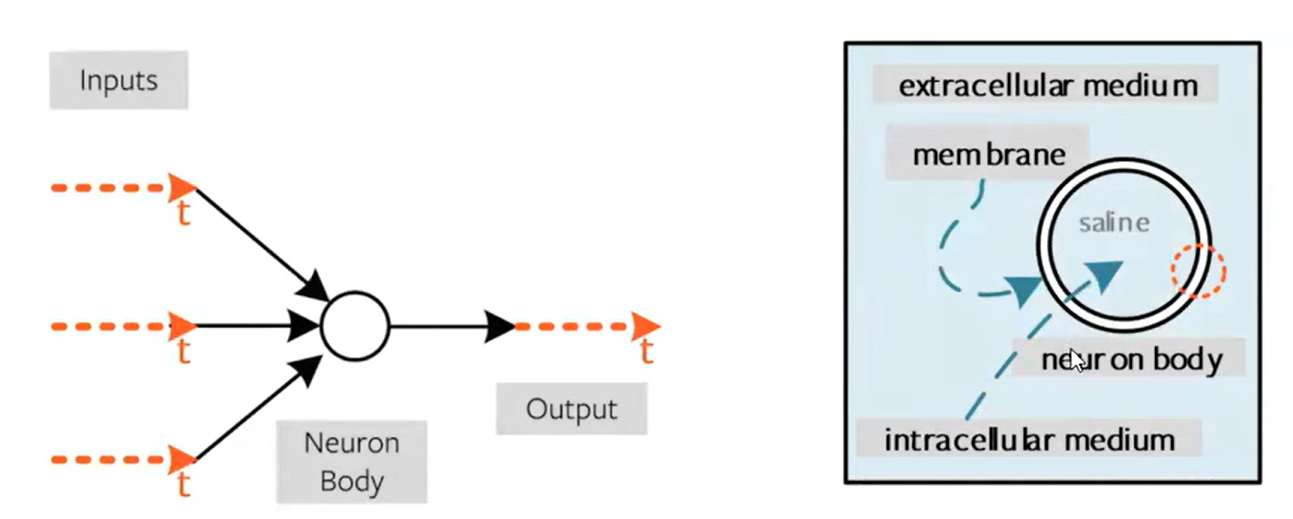

Instantaneous jump in membrane potential followed by a decay. RC circuit: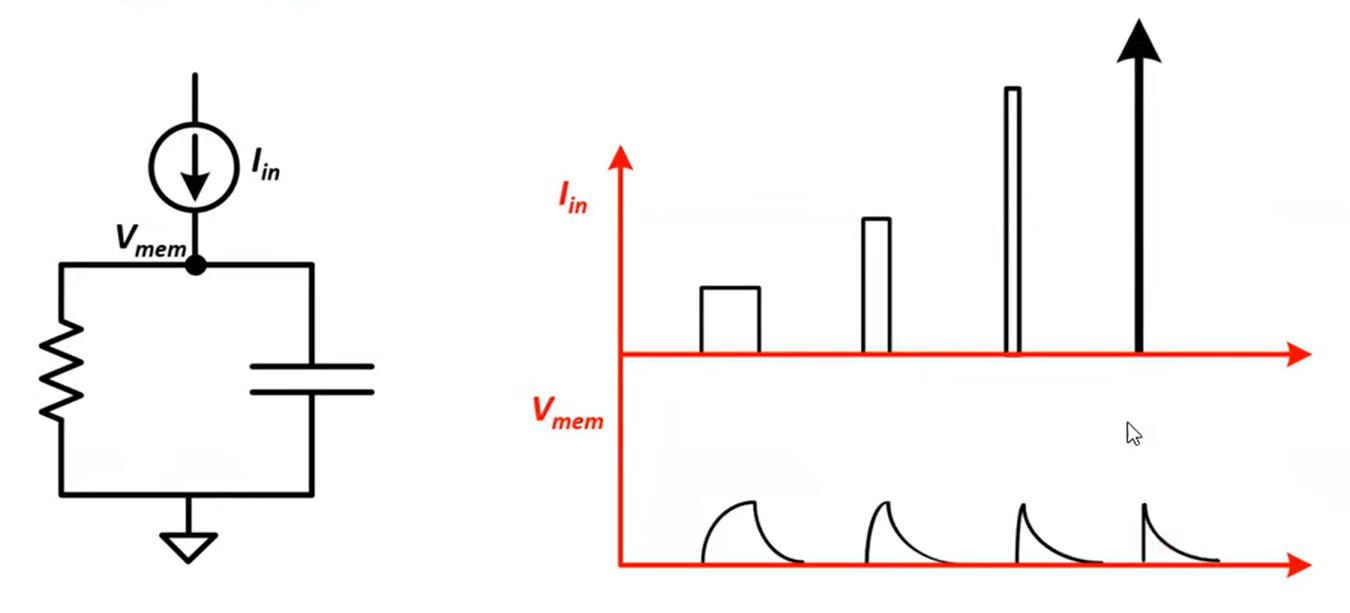

Discretise: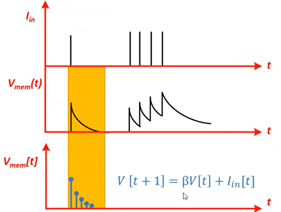

Fire, use the thresholding mechanism.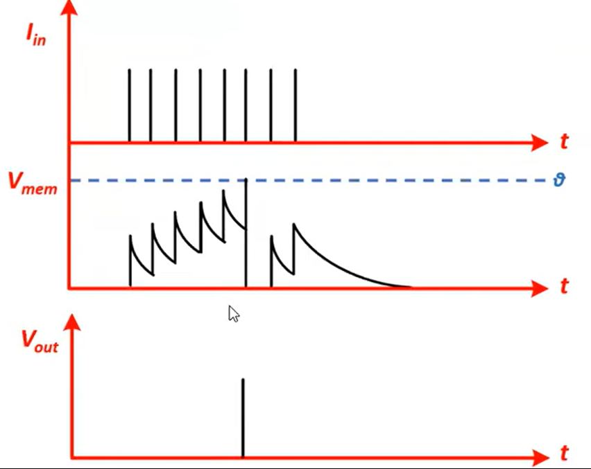

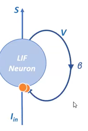
Structure

$$V[t + 1] = \beta V[t] + I_\text{in} [t]$$

$$S[t + 1] = H(V[t+1] - V_{\text{thr}})$$

Calculating the loss

Cross entropy rate loss
Count all spikes at the output and apply CE loss
Maximise correct class count, minimise incorrect class count
MSE count loss
Set a target spike for correct and incorrect classes
MSE Membrane loss
Micromanage the membrane potential at each time step (useful for temporal codes)
L1 sparsity regularisation
Add a penalty term that accumulates all spikes

$$\frac{dL}{dW} = f(\frac{dL}{dS[3]} \frac{dS[3]}{dV[3]} \frac{dV[3]}{dI[3]} \frac{dI[3]}{dW})$$

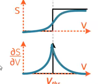
Surrogate gradients

There is the non-differentiability problem: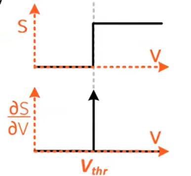

Surrogate gradients approximate the gradient on the backward pass:

Spike operator
Treats the two regions above and below the threshold as two separate operators
Spike-op gradient descent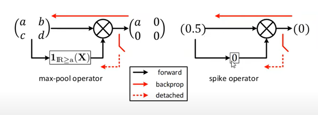

Two approximations are made

• Treating the operator as independent of the input
• The max membrane voltage is the threshold (holds true if each time step is infinitesimally small)

The temporal connections also have a well-defined gradient: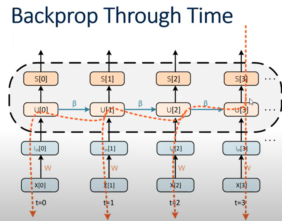

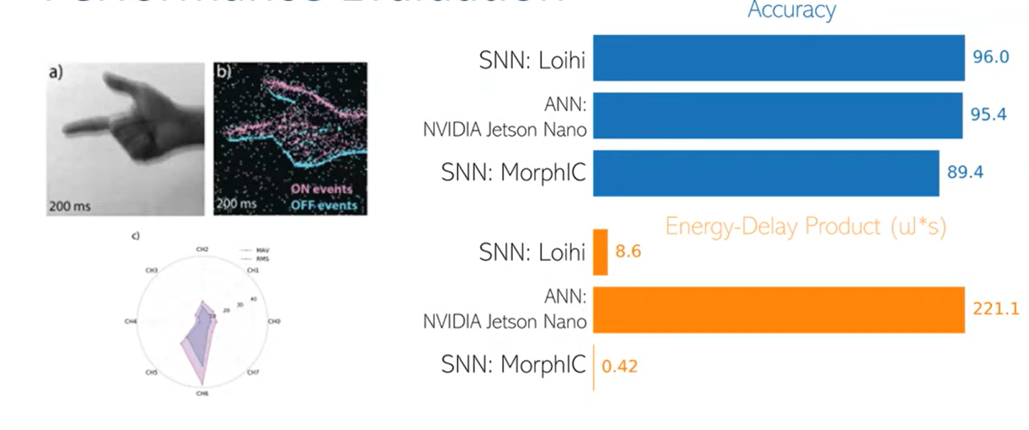
Performance Evaluation

Related work

Attention block

The attention block contains three parts: basic Res-SNN block, shortcut, and CSA module (channel-spatial attention).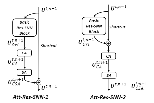

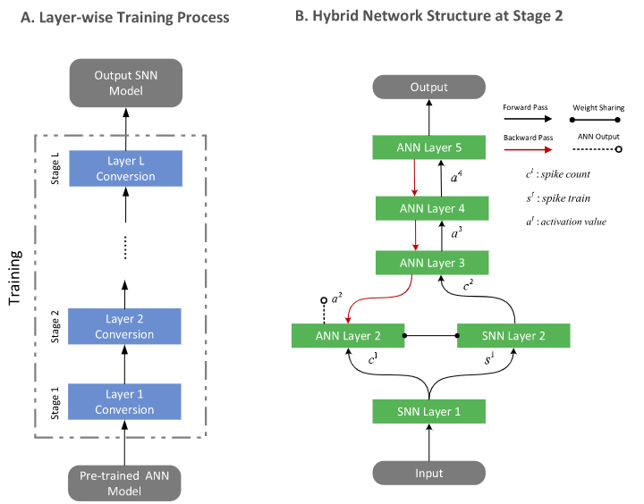
Hybrid network structure

Code

SNNs architecture based on Pytorch:

recurrent_conn = Connection(output_layer, output_layer, w=w_inh_LC)
network.add_layer(input_layer, name="X")
network.add_layer(output_layer, name="Y")
network.add_connection(input_output_conn, source="X", target="Y")
network.add_connection(recurrent_conn, source="Y", target="Y")
spikes = {}
for layer in set(network.layers):
    spikes[layer] = Monitor(network.layers[layer], state_vars=["s"], time=time)
    network.add_monitor(spikes[layer], name="%s_spikes" % layer)
voltages = {}
for layer in set(network.layers) - {"X"}:
    voltages[layer] = Monitor(network.layers[layer], state_vars=["v"], time=time)
    network.add_monitor(voltages[layer], name="%s_voltages" % layer)

Input layer

input_layer = Input(
    shape=[in_channels, input_shape[0], input_shape[1]], traces=True, tc_trace=20
)

def forward(self, x: torch.Tensor) -> None:
    # language=rst
    """
    Abstract base class method for a single simulation step.

    :param x: Inputs to the layer.
    """
    if self.traces:
        # Decay and set spike traces.
        self.x *= self.trace_decay

        if self.traces_additive:
            self.x += self.trace_scale * self.s.float()
        else:
            self.x.masked_fill_(self.s.bool(), self.trace_scale)

    if self.sum_input:
        # Add current input to running sum.
        self.summed += x.float()

Output layer

Leaky integrate and fire (LIF) node:

def forward(self, x: torch.Tensor) -> None:
    # language=rst
    """
    Runs a single simulation step.

    :param x: Inputs to the layer.
    """
    # Decay voltages.
    self.v = self.decay * (self.v - self.rest) + self.rest

    # Integrate inputs.
    x.masked_fill_(self.refrac_count > 0, 0.0)

    # Decrement refractory counters.
    self.refrac_count -= self.dt

    self.v += x  # interlaced

    # Check for spiking neurons.
    self.s = self.v >= self.thresh

    # Refractoriness and voltage reset.
    self.refrac_count.masked_fill_(self.s, self.refrac)
    self.v.masked_fill_(self.s, self.reset)

    # Voltage clipping to lower bound.
    if self.lbound is not None:
        self.v.masked_fill_(self.v < self.lbound, self.lbound)

    super().forward(x)

Adpative LIF node:

def forward(self, x: torch.Tensor) -> None:
    # language=rst
    """
    Runs a single simulation step.

    :param x: Inputs to the layer.
    """
    # Decay voltages and adaptive thresholds.
    self.v = self.decay * (self.v - self.rest) + self.rest
    if self.learning:
        self.theta *= self.theta_decay

    # Integrate inputs.
    self.v += (self.refrac_count <= 0).float() * x

    # Decrement refractory counters.
    self.refrac_count -= self.dt

    # Check for spiking neurons.
    self.s = self.v >= self.thresh + self.theta

    # Refractoriness, voltage reset, and adaptive thresholds.
    self.refrac_count.masked_fill_(self.s, self.refrac)
    self.v.masked_fill_(self.s, self.reset)
    if self.learning:
        self.theta += self.theta_plus * self.s.float().sum(0)

    # voltage clipping to lowerbound
    if self.lbound is not None:
        self.v.masked_fill_(self.v < self.lbound, self.lbound)

    super().forward(x)

Reference

[1] Ponulak, F. and Kasinski, A., 2011. Introduction to spiking neural networks: Information processing, learning and applications. Acta neurobiologiae experimentalis, 71(4), pp.409-433.

[2] Spiking Neural Networks for Image Classification

[3] Training Spiking Neural Networks Using Lessons From Deep Learning

[4] BindsNET/bindsnet

[5] Hazan, H., Saunders, D.J., Khan, H., Patel, D., Sanghavi, D.T., Siegelmann, H.T. and Kozma, R., 2018. Bindsnet: A machine learning-oriented spiking neural networks library in python. Frontiers in neuroinformatics, 12, p.89.

[6] Guo, W., Yantır, H.E., Fouda, M.E., Eltawil, A.M. and Salama, K.N., 2020. Towards efficient neuromorphic hardware: unsupervised adaptive neuron pruning. Electronics, 9(7), p.1059.

[7] Yao, M., Zhao, G., Zhang, H., Hu, Y., Deng, L., Tian, Y., Xu, B. and Li, G., 2023. Attention spiking neural networks. IEEE Transactions on Pattern Analysis and Machine Intelligence.

[8] Wu, J., Xu, C., Han, X., Zhou, D., Zhang, M., Li, H. and Tan, K.C., 2021. Progressive tandem learning for pattern recognition with deep spiking neural networks. IEEE Transactions on Pattern Analysis and Machine Intelligence, 44(11), pp.7824-7840.