Reinforcement means the act of making something stronger, especially a feeling or an idea. So, what kinds of things do we need to make stronger in reinforcement learning? The answer is our learning model, which is considered as policy in reinforcement learning.

Introduction

Reinforcement learning (RL) is the problem faced by an agent that learns behaviour through trail-and-error interactions with a dynamic environment.
Reinforcement learning is an area of machine learning concerned with how intelligent agents out to take actions in an environment to maximise the notion of cumulative reward.
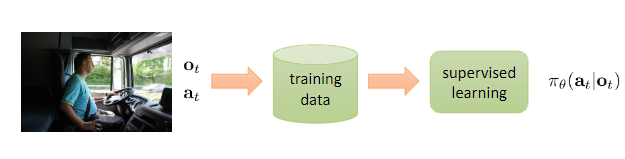
Reinforcement learning differs from supervised learning in not needing labelled input/output pairs to be presented, and in not requiring sub-optimal action to be explicitly corrected. Instead, the focus is on finding a balance between exploration (of uncharted territory) and exploitation (of current knowledge).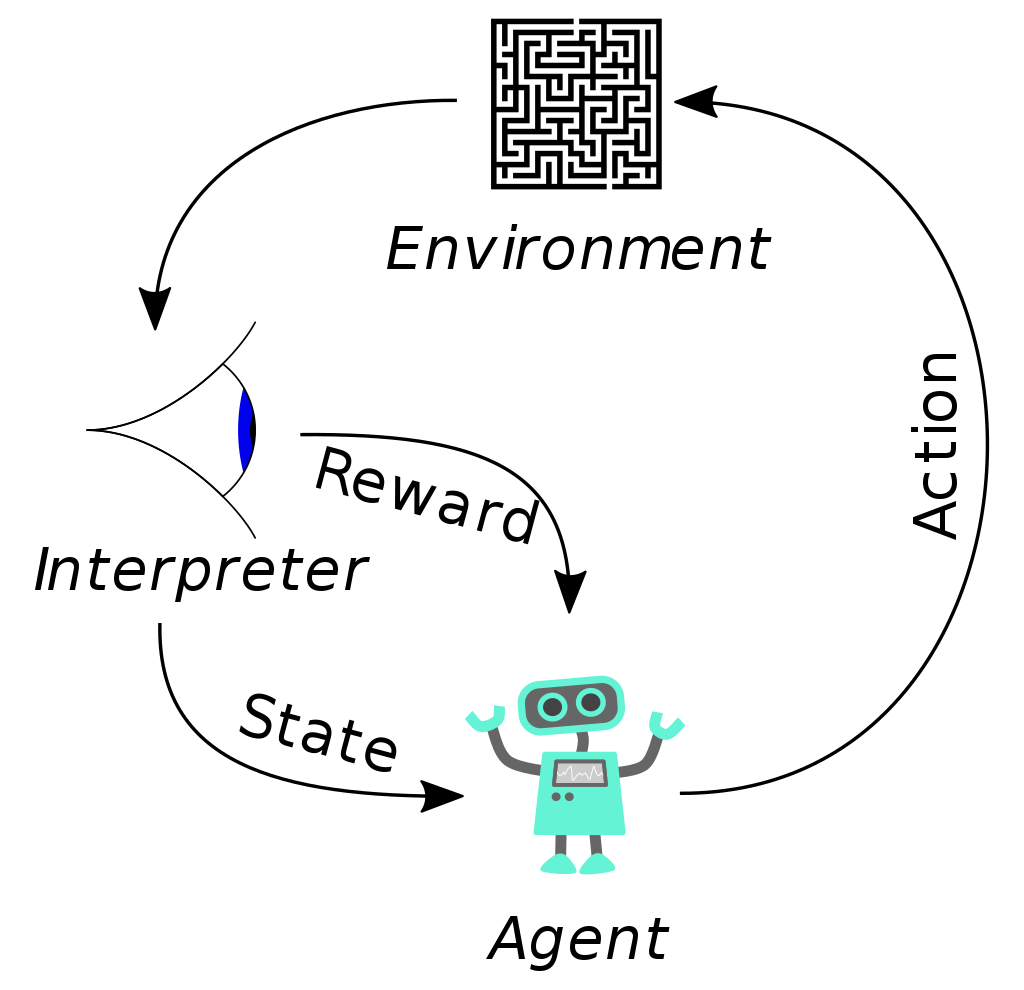

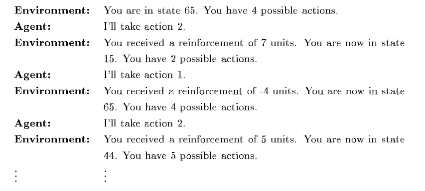
An agent is connected to its environment via perception and action. On each step of interaction, the agent receives as input, $i$, some indication of the current state, $s$, of the environment; the agent then chooses an action, $a$, to generate as output. The action changes the state of the environment, and the value of this state transition is communicated to the agent through a scalar reinforcement signal, $r$. The agent’s behaviour, $B$, should choose actions that tend to increase the long-run sum of values of the reinforcement signal. It can learn to do this over time by systematic trial and error, guided by a wide variety of algorithms that are the subject of later sections of this paper. Input function $I$ determines how the agent views the environment state (identity function, the agent perceives the actual state of the environment).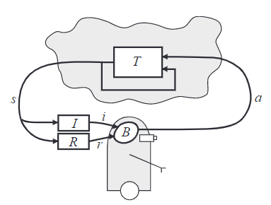

Finally, the model consists of:

• a discrete set of environment states, $S$;
• a discrete set of agent actions, $A$; and
• a set of scalar reinforcement signals; typically {0, 1}, or the real numbers.

The agent’s job is to find a policy $\pi$, mapping states to actions, that maximises some long-run measure reinforcement.

Example - searching for the diamond

The agent should find the best possible path to reach the reward.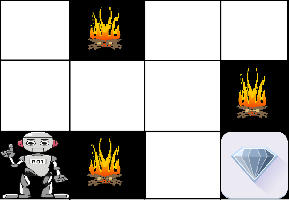

The above image shows the robot, diamond, and fire. The the robot’s goal is to get the diamond reward and avoid the hurdles that are fired. The robot learns by trying all the possible paths and then choosing the path which rewards him with minor limitations. Each right step will give the robot a reward and each wrong step will subtract the reward of the robot. The total reward will be calculated when it reaches the final reward, which is the diamond.

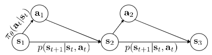
Markov chain

Actually, $s, a, r(s, a), abd p(s^{‘} | s, a)$ define Markov decision process.
Markov chain $M = {S, T}$, transition operator $T$. States $s \in S$, $p(s_{t+1} | s_t)$. Let $\mu_{t, i} = p(s_t = i)$, and $T_{i, j} = p(s_{t + 1} = i|s_t = j)$. $\mu_t$ is a vecotr of probabilities, then $\mu_{t + 1} = T\mu_t$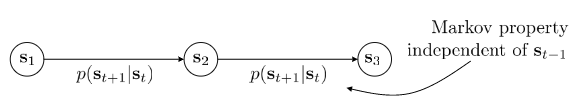

$$M = {S, A ,O, T, \epsilon, r}$$
$S$ Stae space, $A$ action, $O$ observation space, $T$ transition operator(tensor in deep RL), $\epsilon$ emission probability $p(o_t | s_t)$, $r$ reward function, states $s \in S$ (discrete or continuous), actions $a \in A$(discrete or continuous), observations $o \in O$ (discrete or continuous).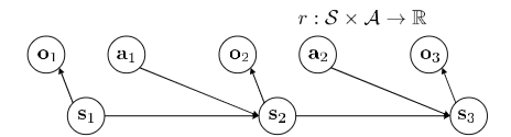

Methodology

There are two main strategies for solving reinforcement-learning problems. The first is to search in the space of behaviours in order to find one that performs well in the environment. The second is to use statistical techniques, and dynamic programming methods to estimate the utility of taking actions in states of the world.

Optimal behaviour
The finite-horizon model is the easiest to think about; at a given moment in time, the agent should optimise its expected reward for the next $h$ steps:
$$E(\sum^{h}_{t=0} r_t)$$

You need not worry about what will happen after that. $r_t$ represents the scalar reward received $t$ steps into the future.
The infinite-horizon discounted model takes the long-run reward of the agent into account, but rewards that are received in the future are geometrically discounted according to discount factor $\gamma$, where ($0 \le \gamma < 1$):
$$E(\sum^{h}_{t=0} \gamma^t r_t)$$

Another optimality criterion is the average-reward model, in which the agent is supposed to take actions that optimise its long-run average reward:
$$\text{lim} _ {h \to \infty} E(\frac{1}{h} \sum^{h} _ {t=0} r_t)$$

Measuring learning performance

• Eventual convergence to optimal. An agent that quickly reaches a plateau at 99% of optimality may, in many applications, be preferable to an agent that has a guarantee of eventual optimality but a sluggish early learning rate.
• Speed of convergence to optimality.
• Regret. A more appropriate measure, then, is the expected decrease in reward gained due to executing the learning algorithm instead of behaving optimally from the very beginning.

Deep reinforcement learning

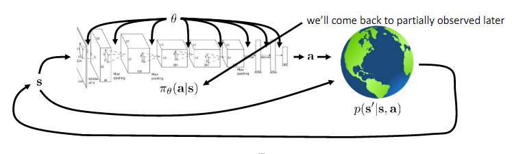
Deep reinforcement learning (deep RL) is a subfield of machine learning that combines reinforcement learning (RL) and deep learning. RL considers the problem of a computational agent learning to make decisions by trial and error. Deep RL incorporates deep learning into the solution, allowing agents to make decisions from unstructured input data without manual engineering of the state space. Deep RL algorithms are able to take in very large inputs (e.g., every pixel rendered to the screen in a video game) and decide what actions to perform to optimise an objective (e.g., maximising the game score).

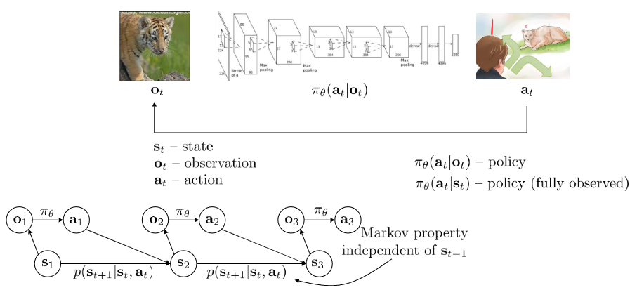
Use a reward function $r(s, a)$ to evaluate which action is good for the policy.

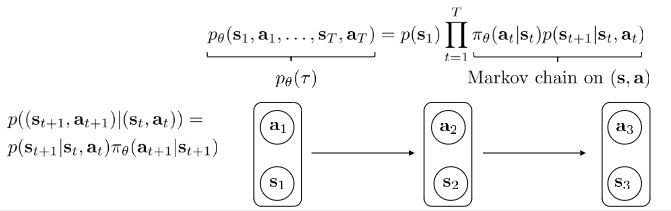
$$p_\theta (s_1, a_1, …, s_T, a_T) = p(s_1) \Pi^{T} _ {t=1} \pi _ \theta (a_t | s_t) p(s_{t+1} | s_t, a_t)$$

$$\theta^{*} = \text{argmax} _ \theta E _ {\tau ~ p_\theta (\tau)} [ \sum_t r(s_t, a_t) ]$$

Infinite horizon case:
$$\theta^{*} = \text{argmax} _ \theta \sum^T _ {t=1} E_{(s_t, a_t) ~ p_\theta (s_t, a_t)} [r(s_t, a_t)]$$

In RL, we almost always care about expectations.

Algorithms

The anatomy of a reinforcement learning algorithm: 1) generate samples; 2) fit a model/estimate the return, 3) improve the policy.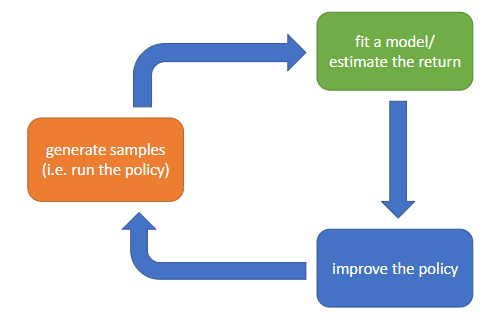

Part 2) often uses Q-functions or value functions. Part 2) can be minimising a loss function (trivial, fast):
$$J(\theta) = E_\pi [\sum_t r_t] \approx \frac{1}{N} \sum^N_{t=1} \sum_t r^i_t$$

Part 3) can be (backprob through $f_\Phi$ and $r$ to train \pi_\theta (s_t) = a_t):
$$\theta \gets \theta + \alpha \nabla_\theta J(\theta)$$

In backprop, part 2) is to learn $f_\Phi$ such that $s_{t+1} \approx f_\Phi (s_t, a_t)$ (expensive).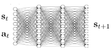

Types of RL algorithms:

1. policy gradients: directly differentiate the above objective
2. value-based: estimate value function or Q-function of the optimal policy (no explicit policy)
3. actor-critic: estimate the value function or Q-function of the current policy, and use it to improve policy
4. model-based RL: estimate the transition model, and then use it for planning, improve a policy or …

Value functions

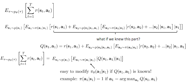
Q function:
Total reward from taking $a_t$ in $s_t$.
$$Q^{pi} (s_t, a_t) = \sum^{T} _ {t^{‘} = t} E_{\pi_\theta} [r(s_{t^{‘}}, a^{t^{‘}}) | s_t, a_t]$$

$$Q^{pi} (s_t, a_t) = E_{a_t ~ \pi(a_t | s_t)} [Q^{\pi} (s_t, a_t)]$$

RL objective:
$$E_{s_1 ~ p(s_1)} | V^{\pi} (s_1)$$

If we have policy $\pi$, and we know $Q^{\pi} (s, a)$, then we can improve $\pi$:
set $\pi^{‘} (a|s) = 1$ if $a = \text{arg max}_a Q^{\pi} (s, a)$
this policy is at least as good as $\pi$.
And it doesn’t matter what $\pi$ is.

Value function:
$$V^{\pi} (s_t) = \sum^{T} _ {t^{‘} = t} E_{\pi_\theta} [r(s_{t^{‘}}, a^{t^{‘}}) | s_t]$$

Compute gradient to increase the probability of good actions $a$:
If $Q^{\pi} (s, a) > V^{\pi} (s)$, then $a$ is better than average. (Recall that $V^{\pi} (s) = E|Q^{\pi} (s, a)|$ under $\pi$(a|s)). Modify $\pi (a | s)$ to increase probability of $a$ if $Q^{\pi} (s, a) > V^{\pi} (s)$.

Deep Q learning

Deep Q learning (DQN):

def learn(self, experiences=None):
    """Runs a learning iteration for the Q network"""
    if experiences is None: states, actions, rewards, next_states, dones = self.sample_experiences() #Sample experiences
    else: states, actions, rewards, next_states, dones = experiences
    loss = self.compute_loss(states, next_states, rewards, actions, dones)

    actions_list = [action_X.item() for action_X in actions ]

    self.logger.info("Action counts {}".format(Counter(actions_list)))
    self.take_optimisation_step(self.q_network_optimizer, self.q_network_local, loss, self.hyperparameters["gradient_clipping_norm"])

Loss:

def compute_loss(self, states, next_states, rewards, actions, dones):
    """Computes the loss required to train the Q network"""
    with torch.no_grad():
        Q_targets = self.compute_q_targets(next_states, rewards, dones)
    Q_expected = self.compute_expected_q_values(states, actions)
    loss = F.mse_loss(Q_expected, Q_targets)
    return loss

Reference

[1] Oxford learner’s Dict, reinforcement
[2] Kaelbling, L.P., Littman, M.L. and Moore, A.W., 1996. Reinforcement learning: A survey. Journal of artificial intelligence research, 4, pp.237-285.
[3] Wiki, Reinforcement learning
[4] Geeksforgeeks, Reinforcement learning
[5] Wiki, Deep reinforcement learning
[6] Sergey Levine, Introduction to Reinforcement Learning.
[7] p-christ/Deep-Reinforcement-Learning-Algorithms-with-PyTorch
[8] Mnih, V., Kavukcuoglu, K., Silver, D., Graves, A., Antonoglou, I., Wierstra, D. and Riedmiller, M., 2013. Playing atari with deep reinforcement learning. arXiv preprint arXiv:1312.5602.