Introduction

Data is biased if certain outcomes are systematically more frequently observed than they would be for a uniformly-at-random sampling procedure. For example, data sampled from a single hospital can be biased with respect to the global population due to differences in living conditions of the local patient population. Can data collected in European hospitals be used to train an intelligent prognosis system for hospitals in Africa?

Domain shift

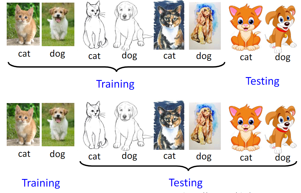
In visual applications, such distribution difference, called domain shift.
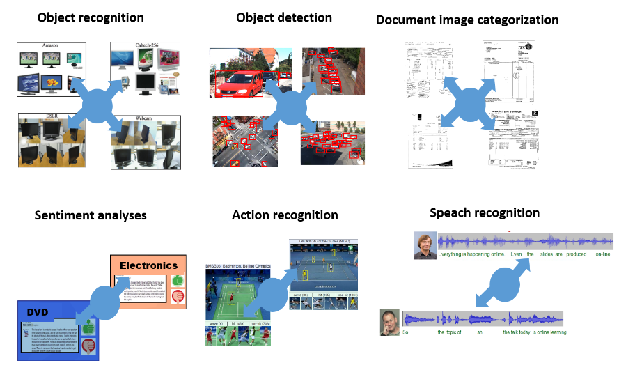
They can be consequences of changing conditions, i.e., background, location, pose changes, but the domain mismatch might be more severe when, for example, the source and target domains contain images of different types, such as photos, NIR images, paintings or sketches.

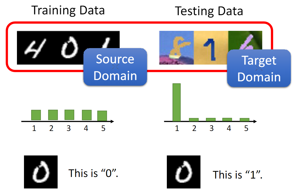
Domain adaptation

Domain adaptation is a particular case of transfer learning that leverages labelled data in one or more related source domains, to learn a classifier for unseen or unlabelled data in a target domain.

Domain generalisation

Domain generalisation (source free domain adaptation) aims to achieve out-of-distribution (OOD) generalisation by using only source data for model learning. Generalisation to OOD data is a capability natural to humans yet challenging for machines to reproduce. This is because most learning algorithm strongly rely on the i.i.d. assumption on source/target data, which is often violated in practice due to domain shift.

Symbol

The model

Assume that the model works with input samples $x\in X$, where $X$ is some input space and certain labels (output) $y$ from the label space $Y$. $Y$ is a finite set ($Y = {1, 2, …, L}$).
There are two distributions, source distribution/domain $\mathcal{S} (x, y)$ and target distribution/domain $\mathcal{T} (x, y)$ on $X\bigotimes Y$.
It can be assumed that $\mathcal{S}$ is “shifted” from $\mathcal{T}$ by some domain shift.
Training examples ${ x_1, x_2, …, x_N }$ are from both the source and the target domains distributed according to the marginal distributions $\mathcal{S}(x)$ and $\mathcal{T} (x)$.

$$\mathcal{S} = {(x_i, y_i)}^n_{i=1} \sim (\mathcal{D}_\mathcal{S})^n$$

$$\mathcal{T} = {x_i}^N_{i = n + 1} \sim (\mathcal{D}_\mathcal{T}^\mathcal{X})^{n^{‘}}$$

Deonte with $d_i$ the binary variable (domain label) for the $i$-th example, which indicates whether $x_i$ come from the source distribution $( x_i \sim \mathcal{S}(x)\ \text{if}\ d_x = 0 )$ or from the target distribution $( x_i \sim \mathcal{T}(x)\ \text{if}\ d_x = 1 )$.
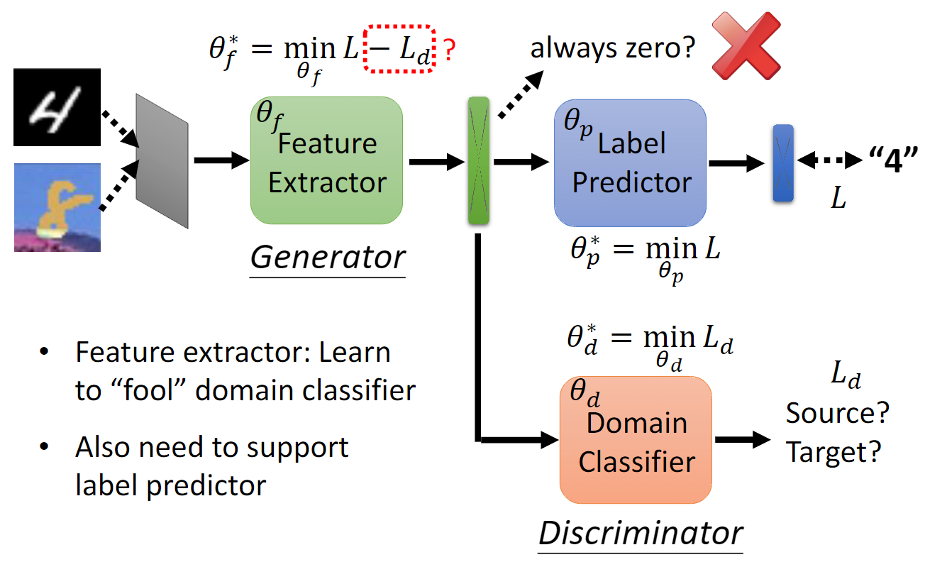
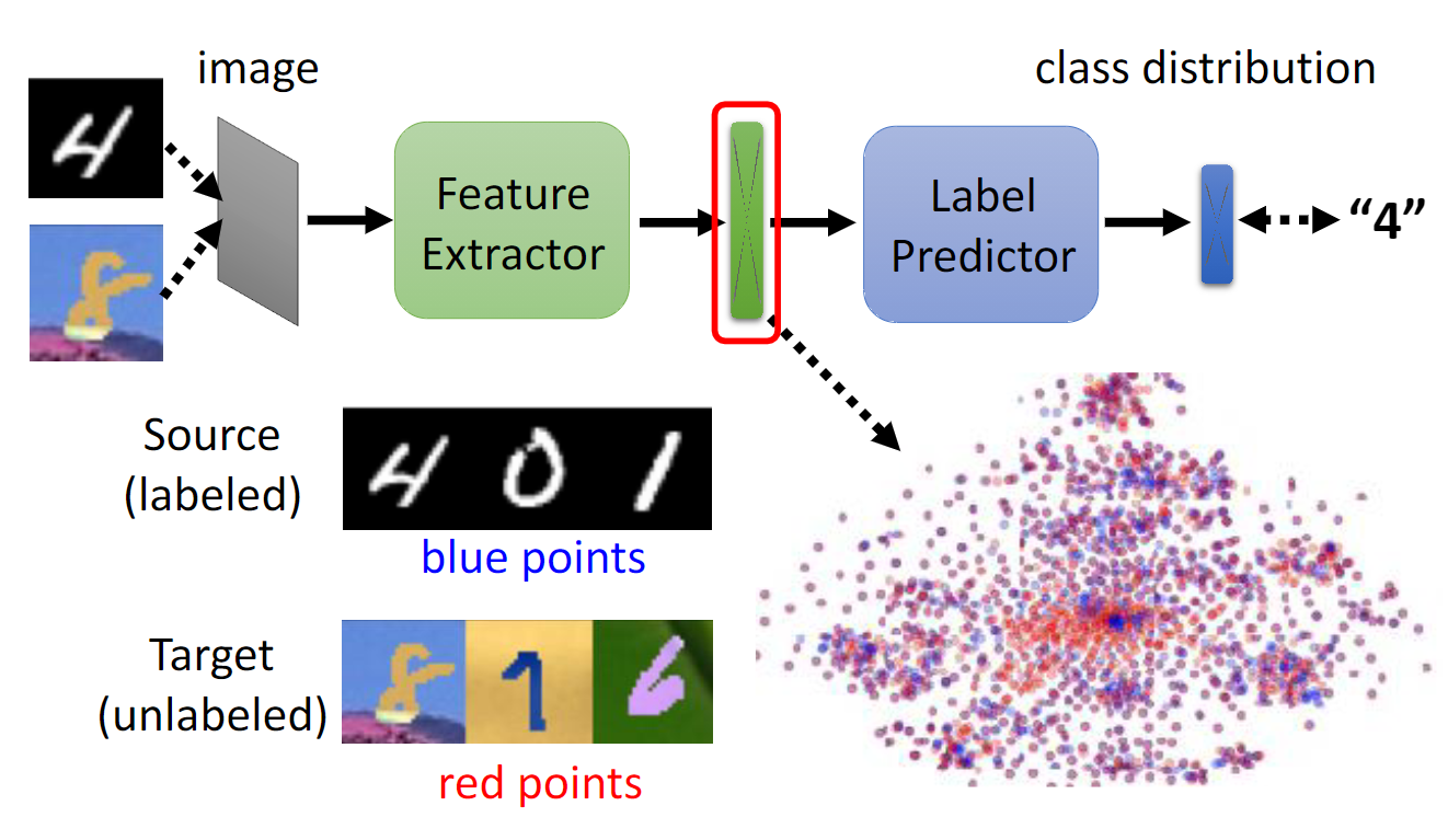
The input $x$ is first mapped by a mapping $G_f$ (a feature extractor) to a $D$-dimensional feature vector $f\in \mathcal{R}^D$. $f$ is the vectors of all layer sin this mapping $\theta_f$, i.e., $f = G_f (x; \theta_f)$.
The feature vector $f$ is mapped by a mapping $G_y$ (label predictor) to the label $y$, and is mapped to the domain label $d$ by a mapping $G_d$ (domain classifier) with the parameters $\theta_d$.
Seek $\theta_f$ that maximises the loss of domain classifier (making two feature distributions as similar as possible, fool the discriminator), $\theta_d$ minimises the loss of domain classifier, and $\theta_y$ minimises the loss of the label predictor:
$$E(\theta_f, \theta_y, \theta_d) = \sum_{i=1, …, N (d_i = 0)} L_y (G_y (G_f (x_i; \theta_f); \theta_y), y_i) - \lambda \sum_{i = 1, …, N} L_d (G_d (G_f (x_i; \theta_f); \theta_d), d_i) =$$
$$\sum_{i=1, …, N (d_i = 0)} L^i_y (\theta_f, \theta_y) - \lambda \sum_{i = 1, …, N} L_d^i (\theta_f, \theta_{d}) $$

Seek $\hat{\theta}_f$, $\hat{\theta}_y$, $\hat{\theta}_d$ that deliver a saddle point of last function:

$$(\hat{\theta}_f, \hat{\theta}_y) = \underset{\theta_f, \theta_y}{\operatorname{argmax}} E(\theta_f, \theta_y, \hat{\theta}_d)$$

$$\hat{\theta}_d = \underset{\theta_d}{\operatorname{argmax}} E(\hat{\theta}_f, \hat{\theta}_y), \theta_d)$$
where $\lambda$ controls the trade-off between the objectives that shape the features during learning.

Optimisation with backpropagation

$$\theta_f \leftarrow \theta_f - \mu \left( \frac{\partial L^i_y}{\partial \theta_f} - \lambda {\partial L^i_d}{\partial \theta_f} \right)$$

$$\theta_y \leftarrow \theta_y - \mu \frac{\partial L^i_y}{\partial \theta_y}$$

$$\theta_d \leftarrow \theta_d - \mu \frac{\partial L^i_d}{\partial \theta_d}$$

where $\mu$ is the learning rate.

Gradient reversal layer is introduced to update $\hat{\theta}_f$, $\hat{\theta}_y$, $\hat{\theta}_d$ efficiently. It doesn’t have parameters.
Assume pseudo-function $R_\lambda (x)$, then $\frac{dR_\lambda}{dx} = -\lambda \mathbf{I}$. So,

$$\hat{E}(\theta_f, \theta_y, \theta_d) = \sum_{i=1, …, N (d_i = 0)} L_y (G_y (G_f (x_i; \theta_f); \theta_y), y_i) + \sum_{i = 1, …, N} L_d (G_d (R_\lambda (G_f (x_i; \theta_f)); \theta_d), d_i) $$

Knowledge storage

• Training a model by source data, then fine-tune the model by target data
• The goal of domain adaptation is to be able to predict labels $y$ given the input $x$ for the target distribution.
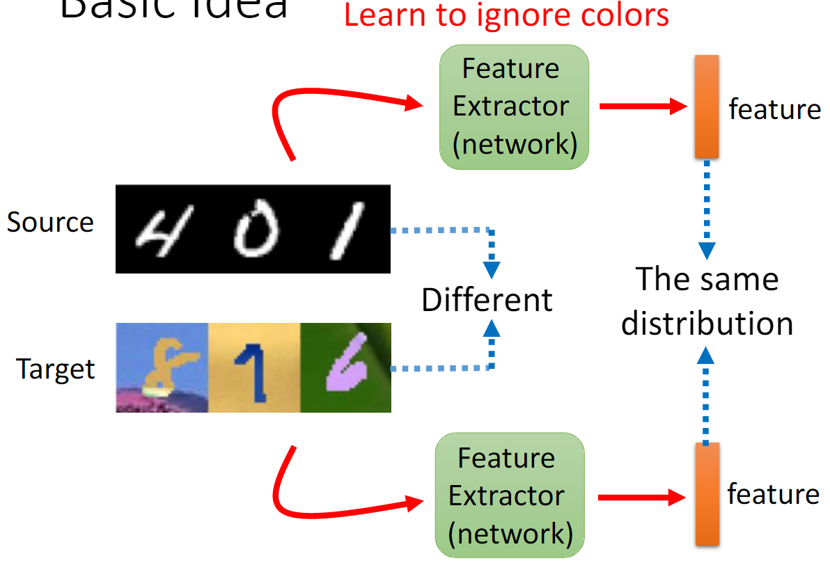
• Make the distributions $\mathcal{S} (f) = {G_f (x; \theta_f) | x \sim \mathcal{S}}$ and $\mathcal{T} (f) = { G_f{x; \theta_f} | x \sim \mathcal{T} (x) }$.
• Make features $f$ domain-invariant.
• One way to estimate the dissimilarity is to look at the loss of the domain classifier $G_d$, provided that the parameters $\theta_d$ of the domain classifier have been trained to discriminate between the two feature distributions in an optimal way.

Only limited target data, so be careful about overfitting.

Sample-based methods

Sample-based methods corrects for biases in the data sampling procedure through individual samples. Methods in this category focus on data importance weighting, or class importance-weighting.

Feature-based methods

Feature-based method focus on reshaping feature space such that a classifier trained on transformed source data will generalise to target data. It can be further divided into several categories: finding subspace mappings, optimal transportation techniques, learning domain invariant representations or constructing corresponding features.

Domain adversarial training

Code:

# domain classifier head
self.domain_classifier = nn.Sequential()
self.domain_classifier.add_module('d_fc1', nn.Linear(50 * 4 * 4, 100))
self.domain_classifier.add_module('d_bn1', nn.BatchNorm1d(100))
self.domain_classifier.add_module('d_relu1', nn.ReLU(True))
self.domain_classifier.add_module('d_fc2', nn.Linear(100, 2))
self.domain_classifier.add_module('d_softmax', nn.LogSoftmax(dim=1))

# loss
err = err_t_domain + err_s_domain + err_s_label

Minimise the difference between blue and red dots

$$ \theta ^ {*} _ {f} = \min _ {\theta_f} L - L_d $$

Feature extractor: learn to “fool” domain classifier

A domain classifier (red) connected to the feature extractor via a gradient reversal layer that multiplies the gradient by a certain negative constant during the backpropagation-based training. Gradient reversal ensures that the feature distributions over the two domains are made similar (i.e., indistinguishable as the domain classifier), thus resulting in the domain-invariant features.
$y_i$ of $x_i$ from the source distribution ($d_i = 0$) is known at training time, otherwise is unknown if from $d_j = 1$.

Limitation

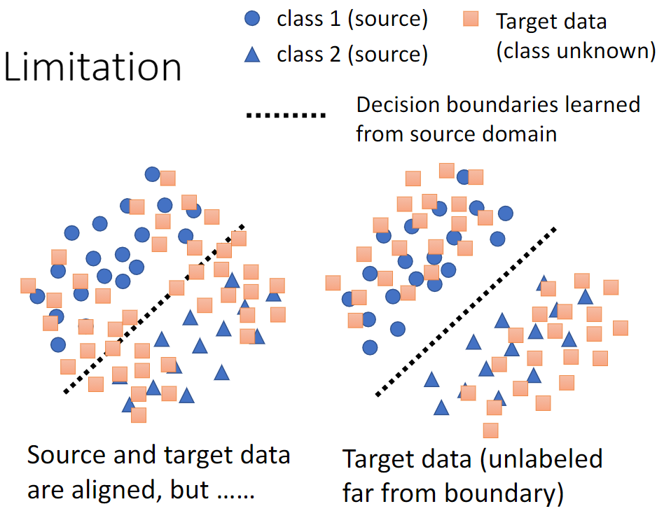
Consider the decision boundary
Far away from boundary vs. Near the boundary

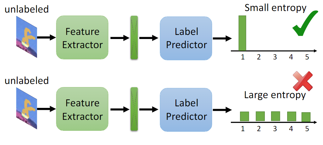
method: DIRT-T, maximum classifier discrepancy

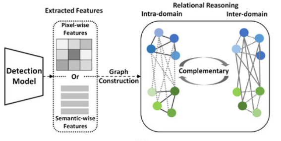
Graph domain adaptation

The method reasons foreground object relationships in both intra- and inter-domain. The graph construction process mines the foreground pixels or regions based on the extracted features.

Intermediate domain construction

The intermediate domain plays as the bridge to gradually reduce distribution divergence across source and target domains.
Maximum structural generation discrepancy (MSGD) estimate and mitigate domain shift via introducing an intermediate domain. MSGD explores the cross-domain structural knowledge over target samples to explicity synthesize an intermediate domain with the specific source samples and utilises it to bridge source and target.

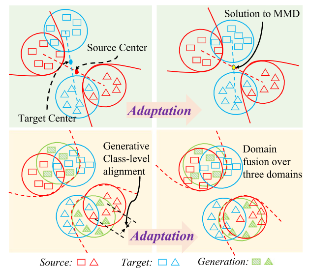
Besides domain level alignment, there is class-level alignment. Class-level alignment can eliminate domain shift across source and intermediate domains due to their semantic similarity.

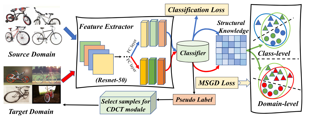
CDD and MMD means the class-level and domain level loss computation tools, respectively. Codes:

# prepare the features
aug_feats = []
feats_toalign_S = self.prepare_feats(feats_source)
feats_toalign_T = self.prepare_feats(feats_target)
similarity_mask = self.block_diag(torch.ones(self.args.num_selected_classes,
                                                self.args.train_class_batch,
                                                self.args.train_class_batch)).cuda()
similarity_st = F.normalize(similarity_mask * torch.cosine_similarity(feats_toalign_S[1].unsqueeze(1), feats_toalign_T[1].unsqueeze(0), dim=2), p=1, dim=1)
aug_feats.append(torch.mm(similarity_st.detach(), feats_toalign_T[0]))
aug_feats.append(torch.mm(similarity_st.detach(), feats_toalign_T[1]))

loss_target_em = self.criterion_em_target(feats_toalign_T[1])
lam = 2 / (1 + math.exp(-1 * 10 * self.loop / 50)) - 1


#msgd loss
cdd_loss_1 = self.cdd.forward(feats_toalign_S, aug_feats,
                source_nums_cls, target_nums_cls)[self.discrepancy_key]
cdd_loss_2 = self.mmd.forward(aug_feats, feats_toalign_T)['mmd']

cdd_alpha = 0.5
cdd_loss = (1-cdd_alpha) * cdd_loss_1 + cdd_alpha * cdd_loss_2 + self.args.em * lam * loss_target_em

cdd_loss *= 0.3
cdd_loss.backward()

cdd_loss_iter += cdd_loss
loss += cdd_loss

Compute the Euclidean distance between source and target domain:

def compute_paired_dist(self, A, B):
    bs_A = A.size(0)
    bs_T = B.size(0)
    feat_len = A.size(1)

    A_expand = A.unsqueeze(1).expand(bs_A, bs_T, feat_len)
    B_expand = B.unsqueeze(0).expand(bs_A, bs_T, feat_len)
    dist = (((A_expand - B_expand))**2).sum(2)
    return dist

Inference-based methods

Inference-based approaches focus on incorporating the adaptation into the parameter estimation procedure. It contains algorithmic robustness, minimax estimators, self-learning, empirical Bayes and PAC-Bayes.

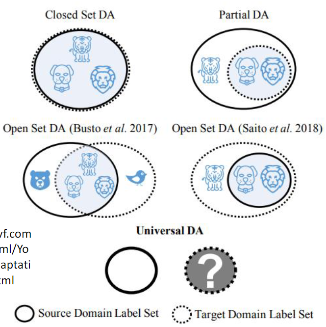
Open set domain adaptation

Open set domain adaptation, closed set domain adaptation

Reference

[1] Zhou, K., Liu, Z., Qiao, Y., Xiang, T. and Loy, C.C., 2022. Domain generalization: A survey. IEEE Transactions on Pattern Analysis and Machine Intelligence.

[2] Csurka, G., 2017. Domain adaptation for visual applications: A comprehensive survey. arXiv preprint arXiv:1702.05374.

[3] Kouw, W.M. and Loog, M., 2019. A review of domain adaptation without target labels. IEEE transactions on pattern analysis and machine intelligence, 43(3), pp.766-785.

[4] ML 2021 Lecture 27: Domain Adaptation

[5] Ganin, Y., Ustinova, E., Ajakan, H., Germain, P., Larochelle, H., Laviolette, F., Marchand, M. and Lempitsky, V., 2016. Domain-adversarial training of neural networks. The journal of machine learning research, 17(1), pp.2096-2030.

[6] Ganin, Y. and Lempitsky, V., 2015, June. Unsupervised domain adaptation by backpropagation. In International conference on machine learning (pp. 1180-1189). PMLR.

[7] fungtion/DANN

[8] Xia, H., Jing, T. and Ding, Z., 2022. Maximum structural generation discrepancy for unsupervised domain adaptation. IEEE Transactions on Pattern Analysis and Machine Intelligence.

[9] HaifengXia/GSP-MSGD