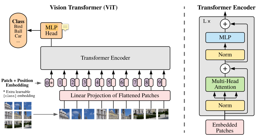
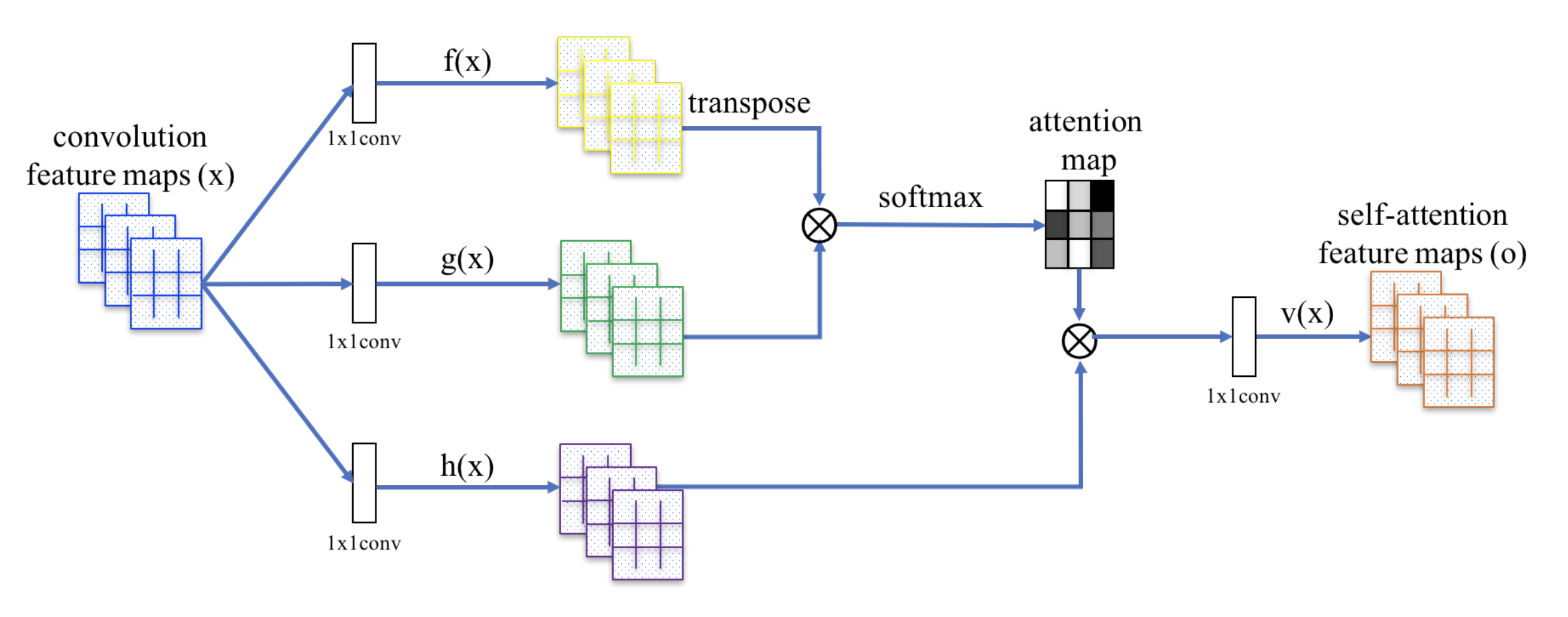
Vision transformer slices the image into patches and uses self-attention mechanisms (inter-patches) (qkv interaction) to process the features.

Vision transformer

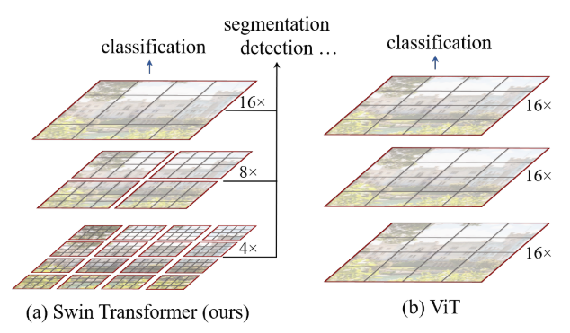
Swin transformer

Shifted window transformer. Merging image patches (shown in gray) in deeper layers. Linear computation complexity to input image size due to computation of self-attention only within each local window (shown in red).

SwinTransformer:
    x = self.PatchEmbed(x)
    if self.ape:
        x = x + self.absolute_pos_embed
    x = self.pos_drop(x)
    for layer in self.layers:
        x = layer(x)
    x = self.norm(x)  # B L C
    x = self.avgpool(x.transpose(1, 2))  # B C 1
    x = torch.flatten(x, 1)

    x = self.Classifier(x)
# BasicLayer
# SwinTransformerBlock + Patch merging

Cyclic shift + partition windows + window attention + merge window + reverse cyclic shift + FFN:

SwinTransformerBlock:
    # cyclic shift
    if self.shift_size > 0:
        shifted_x = torch.roll(x, shifts=(-self.shift_size, -self.shift_size), dims=(1, 2))
    else:
        shifted_x = x
    # partition windows
    x_windows = windowPartition(shifted_x, self.window_size)  # nW*B, window_size, window_size, C
    x_windows = x_windows.view(-1, self.window_size * self.window_size, C)  # nW*B, window_size*window_size, C
    # W-MSA/SW-MSA
    attn_windows = self.attn(x_windows, mask=self.attn_mask)  # nW*B, window_size*window_size, C
    # merge windows
    attn_windows = attn_windows.view(-1, self.window_size, self.window_size, C)
    shifted_x = windowReverse(attn_windows, self.window_size, H, W)  # B H' W' C
    # reverse cyclic shift
    if self.shift_size > 0:
        x = torch.roll(shifted_x, shifts=(self.shift_size, self.shift_size), dims=(1, 2))
    else:
        x = shifted_x
    x = x.view(B, H * W, C)
    # FFN
    x = shortcut + self.drop_path(x)
    x = x + self.drop_path(self.mlp(self.norm2(x)))

Shifted window:
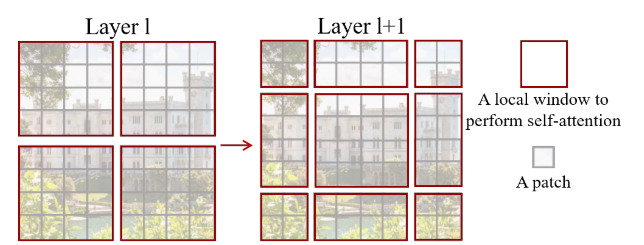
For crossing the boundary, change the size of windows (通過變換窗口大小達到cross boundary的效果).
Layer l: self-attention is computed within each window
Layer l+1: self-attention computation in the new windows crosses the boundaries of the previous windows in layer l, providing connections among them

h_slices = (slice(0, -self.WindowSize),
                        slice(-self.WindowSize, -self.shift_size),
                        slice(-self.shift_size, None))
w_slices = (slice(0, -self.WindowSize),
            slice(-self.WindowSize, -self.shift_size),
            slice(-self.shift_size, None))

Patch merging:

# input
torch.Size([3, 3136, 96])
# split image res
torch.Size([3, 56, 56, 96])
# downsize image res into 4 channel
torch.Size([3, 28, 28, 384])
# merge image res
torch.Size([3, 784, 384])
# reduction
torch.Size([3, 784, 192])

windowPartition: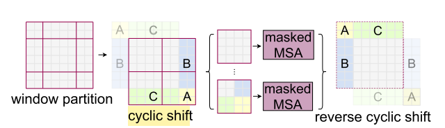

# Input
torch.Size([1, 56, 56, 1])
# PatchesRes split into 4
torch.Size([1, 8, 7, 8, 7, 1])
# Window
torch.Size([64, 7, 7, 1])
# (num_windows*B, WindowSize, WindowSize, C)

windowReverse:

# windows.shape
torch.Size([192, 7, 7, 96])
# Split num_ win * B into batchsize and two  H // window size 
torch.Size([3, 8, 8, 7, 7, 96])
# merge window size and  H // window size into PatchesRes
torch.Size([3, 56, 56, 96])

QKV

196 is the number of patches, 768 is the patches ensemble size, Q K V directly handles this tensor.
Original:

x.shape
torch.Size([3, 3, 224, 224])
Patch embedding:
x.shape
torch.Size([32, 197, 768])

Dimension of q, k, v is the same:

Query.shape
torch.Size([32, 12, 197, 64])
Key.shape
torch.Size([32, 12, 197, 64])
Value.shape
torch.Size([32, 12, 197, 64])
x.shape
torch.Size([32, 12, 197, 197])

Token

An additional [class] token (image representation).
It is not really important. However, we wanted the model to be “exactly Transformer, but on image patches,” so we kept this design from Transformer, where a token is always used.

x.shape
torch.Size([3, 196, 768])
ClassTokens.shape
torch.Size([3, 1, 768])
x.shape
torch.Size([3, 197, 768])

Token classes are common practice in NLP where you have one token that pools information from the rest of the tokens through rounds of attention, usually to classify the sentence at the end. Whether it is completely necessary for ViT to work is up for debate. My take is it isn’t that important. You could pool all the embeddings from the last layer and probably still get great results at scale.

MLP layer

A multilayer perceptron (MLP) is a feedforward artificial neural network (ANN) class. The term MLP is used ambiguously, sometimes loosely to mean any feedforward ANN, sometimes strictly to refer to networks composed of multiple layers of perceptrons (with threshold activation); see § Terminology. Multilayer perceptrons are sometimes colloquially referred to as “vanilla” neural networks, especially when they have a single hidden layer.
An MLP consists of at least three layers of nodes: an input layer, a hidden layer, and an output layer.

Transformer 的 MLP：兩層linear

self.fc1 = nn.Linear(in_features, hidden_features)
self.act = act_layer()
self.fc2 = nn.Linear(hidden_features, out_features)
self.drop = nn.Dropout(drop)

Data structure

Input: reshape the image $x \in R^{H\times W\times C}$ into a sequence of flattened 2D patches $x_p \in R^{N \times (P^2 \dot C)}$.
$(P, P)$ is the resolution of each image patch.
$N = HW/P^2$ is the number of patches
Patch embedding: image to patch, 224x224 to 16 x 16
Position embedding: 3 dimensions to 2 dimensions (+1 dimension if in batch)

Shortcoming

It doesn’t work well for a small dataset without pretrained in the large dataset (ImageNet 1k):
E.g., mobilenetv3 large got 0.89 accuracy, but efficientvitxs got 0.58 accuracy in epoch 70 - 90

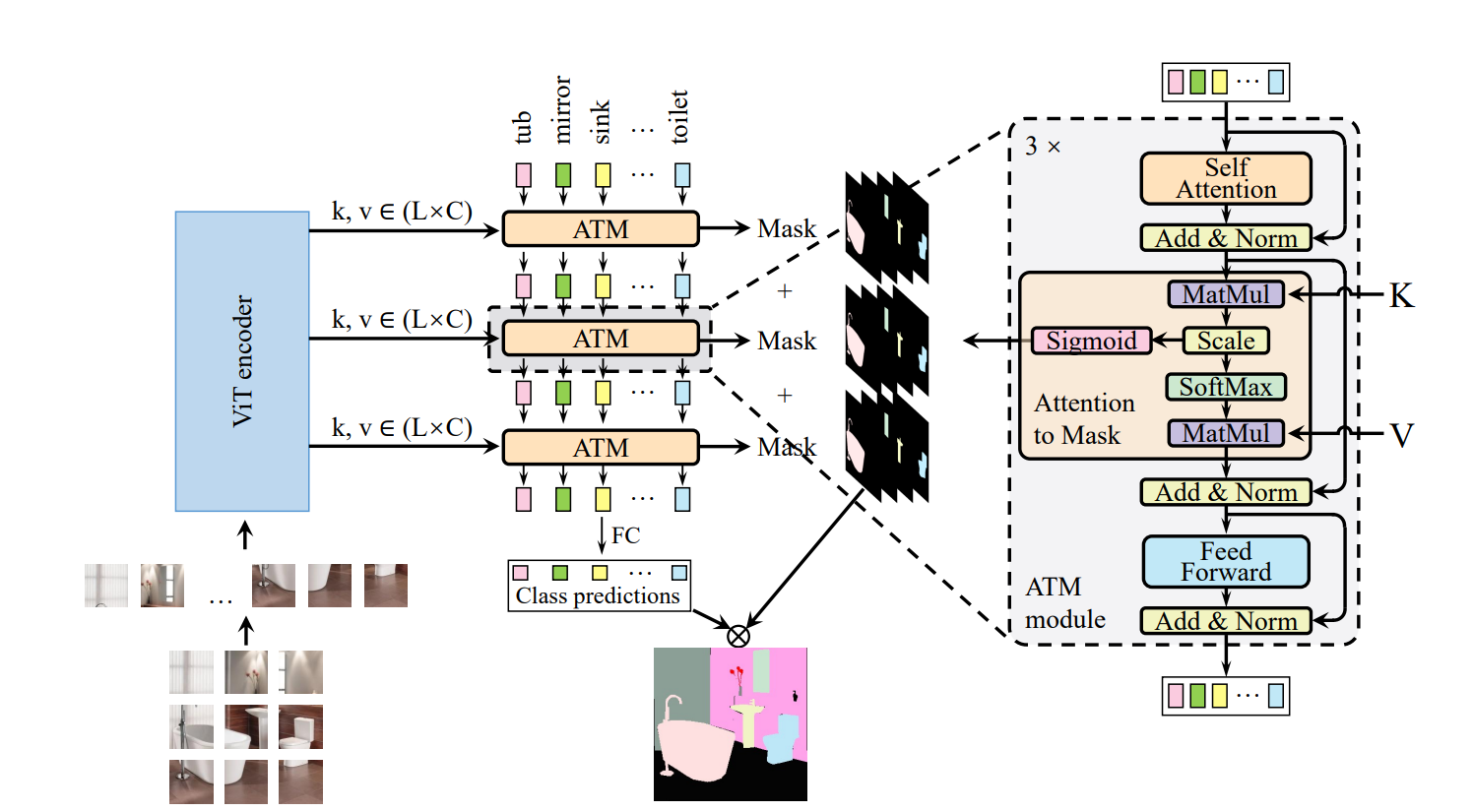
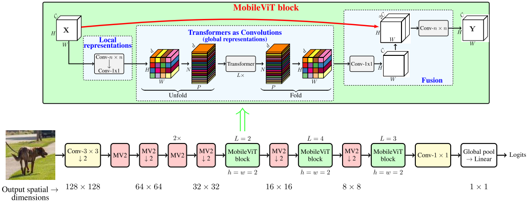
Mobile ViT

MobileViT block replaces local processing in convolutions with global processing using transformers.

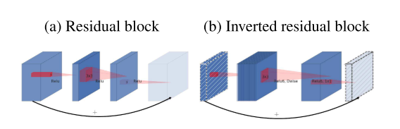
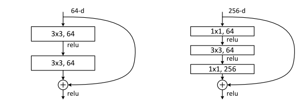
Bottleneck

Classical residuals connect the layers with a high number of channels, whereas inverted residuals connect the bottlenecks. This module takes as an input a low-dimensional compressed representation which is first expanded to a high dimension and filtered with a lightweight depthwise convolution.

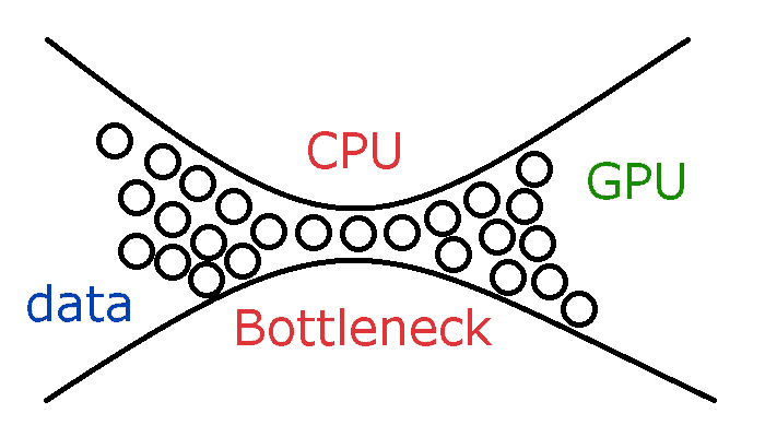
Kaiming He et al. used a bottleneck block, in which the middle operation contributes to smaller channels on the middle part.

spatial inductive biases (Conv weight has bias)

An inductive bias also known as learning bias, of a learning algorithm is the set of assumptions the leaner uses to predict outputs or given inputs that it has not encountered.

Local representation

Given $H \times W \times C$ tensor, MobileViT applies a $n\times n$ standard convolution layer followed by a point-wise (or $1 \times 1$) convolution layer to produce $H \times W \times d$ tensor. The first operation is used to encode local spatial information, and the second one is used to project the tensor to a high-dimension space ($d$ dimension, $d>C$).

Global representaion

The global info is encoded by learning inter-patch info by using transformers.
Local: among pixels (a small area of image)
Global: among patches (a whole area of image)

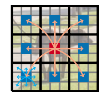
Global + local:
The red pixel can aggregate information from all pixels using local (cyan-colored arrows) and global (orange-colored arrows) information.

Reference

[1] Is the extra class embedding important to predict the results, why not simply use feature maps to predict?

[2] Whats the point of the class token here?

[3] Multilayer perceptron

[4] Vaswani, A., Shazeer, N., Parmar, N., Uszkoreit, J., Jones, L., Gomez, A.N., Kaiser, Ł. and Polosukhin, I., 2017. Attention is all you need. In Advances in neural information processing systems (pp. 5998-6008).

[5] Wiki: Inductive bias

[6] Howard, A., Sandler, M., Chu, G., Chen, L.C., Chen, B., Tan, M., Wang, W., Zhu, Y., Pang, R., Vasudevan, V. and Le, Q.V., 2019. Searching for mobilenetv3. In Proceedings of the IEEE/CVF international conference on computer vision (pp. 1314-1324).

[7] Mehta, S. and Rastegari, M., MobileViT: Light-weight, General-purpose, and Mobile-friendly Vision Transformer. In International Conference on Learning Representations.