When your input data has a large scale, then probably, you are supposed to think about how to speed up gradient descent processes of your learning systems.

Types of gradient descent

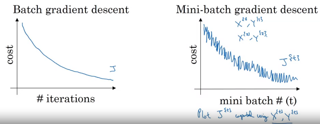
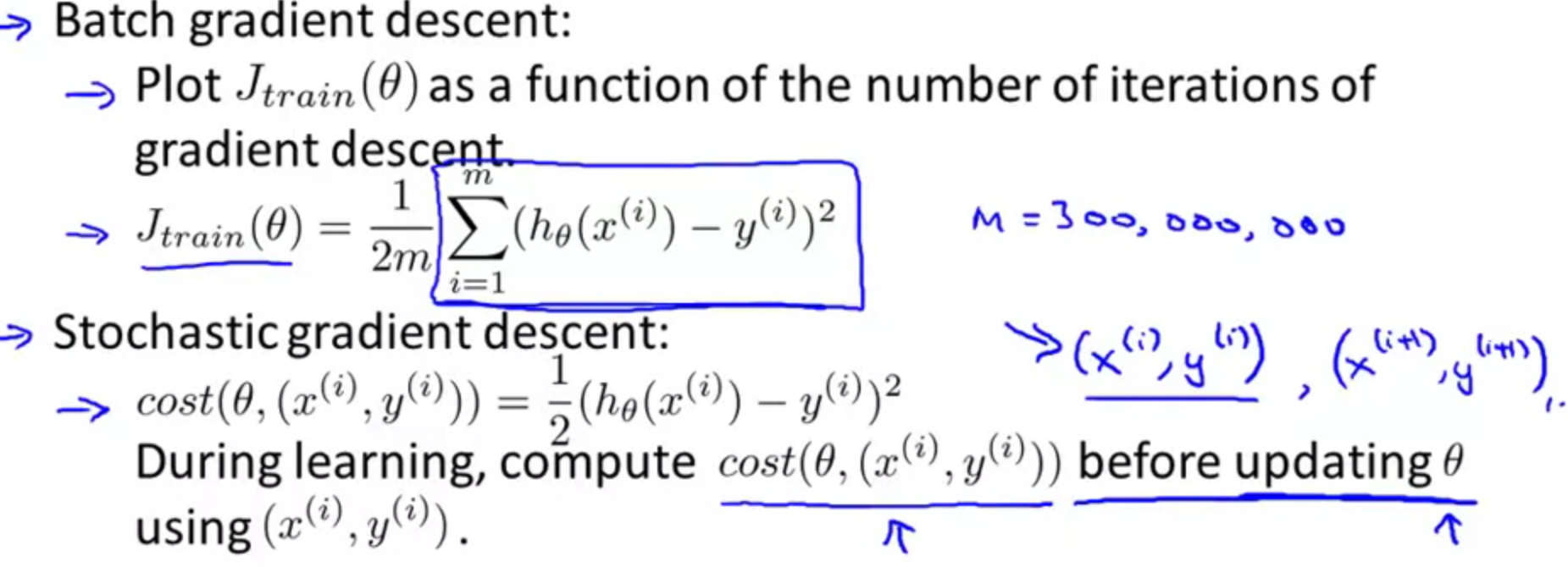
Batch gradient descent

Use all m examples in each iteration.

Stochastic gradient descent

Characteristics

• Use all 1examples in each iteration.
• One of the advantages of stochastic gradient descent is that it can start progress in improving the parameters $\theta$ after looking at just a single training example; in contrast, batch gradient descent needs to take a pass entire training set before it starts to make progress in improving the parameters‘ values.
• In each iteration of stochastic gradient descent, the algorithm needs to examine/use only one training example.
• Before running stochastic gradient descent, you should randomly shuffle (reorder) the training set.
• One of the advantages of stochastic gradient descent is that it uses parallelization and thus runs much faster than batch gradient descent.
• If you have a huge training set, then stochastic gradient descent may be much faster than batch gradient descent.
• Lose speedup from vectorization.

Steps

• Randomly shuffle dataset
• Repeat minimize cost function

vs. Batch gradient descent

For every 1000 iterations (maybe), plot $cost(\theta, (x^{(i)}, y^{(i)}))$ averaged over the last 1000 examples processed by an algorithm. Increase the number of iterations can lower noise.

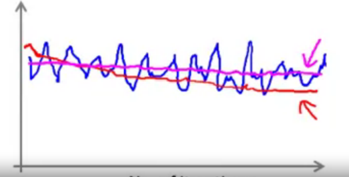
Learning rate $\alpha$ is typically held constant. Can slowly decrease \alpha over time if we want \theta to converge. eg. $\alpha = \frac{const1}{iteration_times + const2}$

Mini-batch gradient descent

Use all b examples in each iteration.

Say $b = 10$, $m = 1000$.

Repeat{

for $i = 1, 11, 21, 31, …, 991$

$${\theta_j := \theta_j - \alpha \frac{1}{10}\sum^{i+9}_{k=i}(h_\theta (x^{(x)}) - y^{(k)}) x_j^{(k)}, \text{for every} \ j = 0, …, n }$$

}

Mini-batch t: $X^{ {t} }, T^{ {t} }$

Forward:
$$Z^{[1]} = W^{(1)} X^ + b^{[1]}$$
$$A^{[1]} = g^{[1]} (Z^{[1]})$$
….
$$A^{[L]} = g^{[L]} (Z^{[L]})$$

Compute cost:

$$J^{(t)} = \frac{1}{1000} \sum^l_{i = 1} L(\hat{y}^{(i)}, y^{(i)}) + \frac{\lambda}{2m} \sum_l {||W^{[l]}||} ^2_F$$

Backprop to compute gradients cost $J^{ {t} }$:
$$W^{[l]}:= W^{[l]} - \alpha dW^{[l]}, b^{[l]}:= b^{[l]} - \alpha db^{[l]}$$

If mini-batch size = m: Batch gradient descent
If mini-batch size = 1: Stochastic gradient descent

Characteristics

• Less computation is used to update the weights.
• Computing the gradient for many cases simultaneously uses matrix-matrix multipliers which are very efficient especially on GPUs.

For large neural networks with very large and highly redundant training sets, it is nearly always best to use mini‐batch learning.

How to choose your mini-batch size
If small training set: use batch gradient descent ($m \leq 2000$)
Typical mini-batch sizes: (common)$2^6 = 64, 2^7, 2^8, 2^9 , 2^10$
Make sure mini-batch fit in CPU/GPU memory, $X^, Y$

Steps

• Guess an initial learning rate
• Write a simple program to automate this way of adjusting the learning rate
• Turn down the learning rate when the error stops decreasing

Online learning

Online learning is the process of answering a sequence of questions given (maybe partial) knowledge of the correct answers to previous questions and possibly additional available information.

Characteristics

• Can adapt to changing user preference.

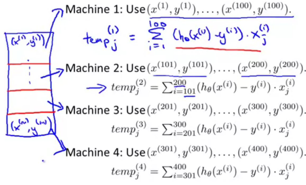
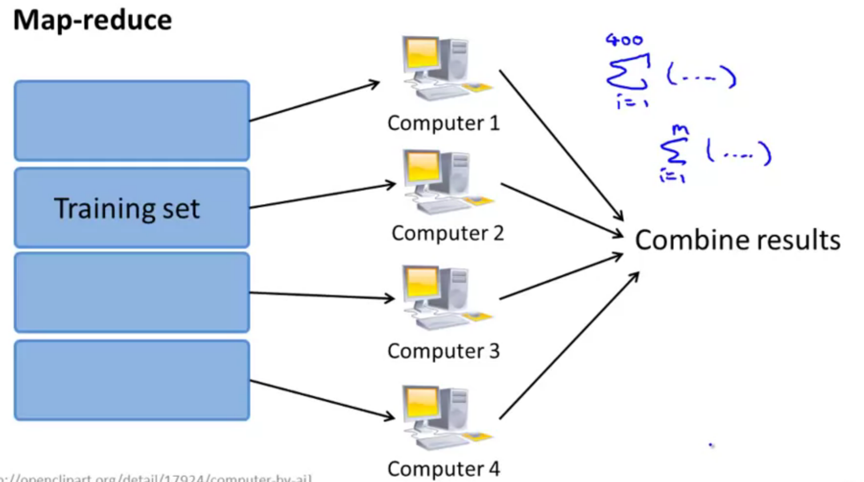
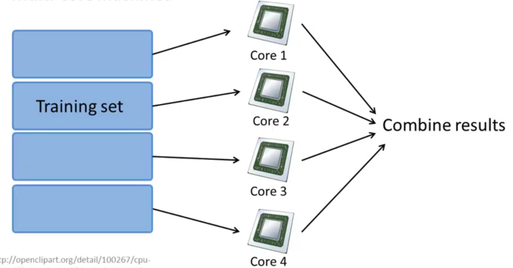
Map-reduce and data parallelism

For batch gradient descent. Many learning algorithms can be expressed as computing sums of functions over the training set, if not, you can not use this algorithm for your gradient descent processes. It is also work in multi-core machines.

Combine:

$$\theta_j = \theta_j - \alpha \frac{1}{m} (temp_j^{(1)} + temp_j^{(2)} + temp_j^{(3)} + temp_j^{(4)})$$

Class exercises

Homework

Q4: Assuming that you have a very large training set, which of the following algorithms do you think can be parallelized using map-reduce and splitting the training set across different
machines? Check all that apply.

Logistic regression trained using stochastic gradient descent.

- [x] Computing the average of all the features in your training set $\mu = \frac{1}{m} \sum^m_{i=1} x^{(i)}$ (say in order to perform mean normalization).

Linear regression trained using stochastic gradient descent.

- [x] Logistic regression trained using batch gradient descent.

Q5: Which of the following statements about map-reduce are true? Check all that apply.

- [x] If you have only 1 computer with 1 computing core, then map-reduce is unlikely to help.

- [x] Because of network latency and other overhead associated with map-reduce, if we run map-reduce using N computers, we might get less than an N-fold speedup compared to using 1 computer.

When using map-reduce with gradient descent, we usually use a single machine that accumulates the gradients from each of the map-reduce machines, in order to compute the parameter update for that iteration.

If we run map-reduce using N computers, then we will always get at least an N-fold speedup compared to using 1 computer.

Reference

[1] Andrew NG, Machine learning

[2] Hinton, G., Srivastava, N. and Swersky, K., 2012. Neural networks for machine learning lecture 6a overview of mini-batch gradient descent. Cited on, 14(8).

[3] Shalev-Shwartz, S., 2011. Online learning and online convex optimization. Foundations and Trends in Machine Learning, 4(2), pp.107-194.